"OpenCV insists I am BGR, Pillow swears I am RGB, and scikit-image quietly converted me to float64 while nobody was looking. I just lie here, contiguous in memory, and let them argue."
A Diplomatically Neutral NumPy Array
The four major Python imaging libraries are not competitors but complements: each one optimizes a different corner of the same job, and the professional move is to know which corner you are standing in. OpenCV optimizes speed and breadth, scikit-image optimizes clarity and scientific correctness, Pillow optimizes file I/O and simplicity, and SciPy ndimage optimizes n-dimensional generality. They interoperate through one shared currency, the NumPy array, and nearly every bug at their borders is a conversion bug.
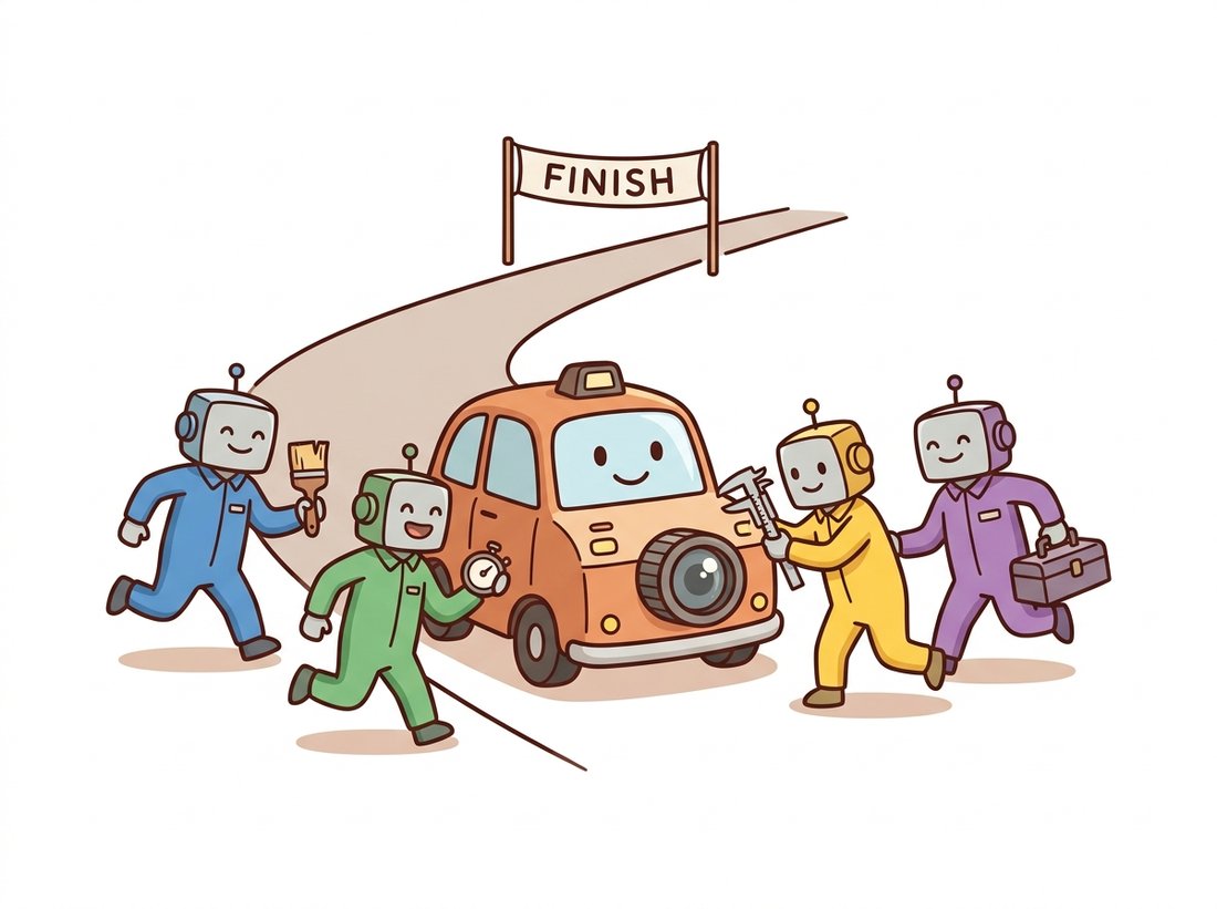
Pick the wrong library for a task and you do not get an error; you get faces that render blue, denoisers that return black, and unit tests that pass on the grayscale fixture and lie about the color one. Throughout Part I we reached for whichever library had the cleanest API for the moment: Pillow to load files in Chapter 0, OpenCV for warps in Chapter 5, scikit-image for denoisers in Chapter 7. This section finally puts the four side by side so those silent failures stop happening: where each came from, what data model it assumes, how to translate between them safely, and a decision procedure for choosing. By the end you will reach for the right library on reflex and cross between them without ever swapping a channel by accident. Treat it as the reference you return to whenever an import decision feels arbitrary. Think of this chapter as the pit stop at the end of Part I, where the whole imaging toolkit gets bolted on at once (see the illustration below).
1. Four Libraries, Four Philosophies Beginner
OpenCV (cv2) is a C++ library wearing a Python costume. Born at Intel in 1999, it grew into one of the largest open-source vision codebases in existence: thousands of functions spanning image processing, video I/O, calibration, tracking, and legacy machine learning. Its Python bindings hand you NumPy arrays, but the semantics underneath are C++: preallocated outputs, in-place options, integer-first dtypes, and the famous BGR channel order it inherited from early Windows bitmap conventions. When raw speed on a CPU matters, OpenCV is usually the answer; Section 8.2 quantifies why.
scikit-image (skimage) is the scientific community's counterproposal: pure-Python-plus-Cython, NumPy-native, with an API designed to read like the textbook. Functions are named after the algorithm and its author (filters.frangi, restoration.richardson_lucy), default to float images in $[0, 1]$, and favor correctness and documentation over raw throughput. Its docs double as a small image processing course, and many functions cite the paper they implement.
Pillow (PIL) is the elder of the family, the maintained fork of the 1995 Python Imaging Library. Its center of gravity is file handling: it reads and writes dozens of formats, understands EXIF orientation, color profiles, animated GIFs, and 16-bit TIFFs, and exposes a friendly Image object with methods like resize and crop. It is the default tool of web backends and the loader underneath torchvision, which is why it reappears in Chapter 18.
SciPy ndimage (scipy.ndimage) is the quiet generalist. It implements filters, morphology, interpolation, and measurements for arrays of any dimensionality, which makes it the only choice in this lineup when your "image" is a 3D microscopy stack or a 4D fMRI volume. Its API is spartan, but several scikit-image functions delegate to it internally, and its map_coordinates is the engine behind many custom warps. Figure 8.1.1 places all four on the common NumPy foundation.
Table 8.1.1 compresses the comparison into the form you will actually use: a row to scan before you type import.
| Library | Native image model | Color order | Backend | Strongest at | Weakest at |
|---|---|---|---|---|---|
OpenCV (cv2) | uint8 ndarray (also float32) | BGR | C++, SIMD, IPP, threads | speed, video, breadth | API consistency, docs depth |
| scikit-image | float64 ndarray in [0, 1] | RGB | Python + Cython | clarity, scientific rigor | throughput, video |
| Pillow | Image object with mode | RGB | C (libjpeg, zlib, ...) | file formats, metadata | numeric processing |
| SciPy ndimage | any-dtype, any-dim ndarray | none (no color rules) | C | 3D/4D volumes, generic filters | color handling, I/O |
2. The Data-Model Trap: dtype, Range & Channel Order Intermediate
The libraries agree on the container and disagree on the contents. As established in Chapter 1, an image is an array plus an interpretation, and each library bakes in a different interpretation. A single phrase captures the whole section: interoperation is cheap, interpretation is where bugs live. Those interpretation bugs all live on three axes, worth memorizing as a checklist of three questions to ask at every library border, order, range, axes: which channel order, what value range, and whose coordinate axes?
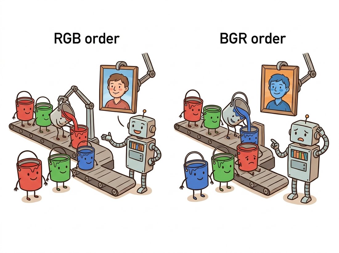
- Channel order. OpenCV stores color as BGR; everyone else uses RGB. Display an OpenCV-loaded photo with Matplotlib and faces turn avatar-blue, as the illustration below makes vivid.
- Dtype and range. OpenCV and Pillow think in
uint8with values 0 to 255; scikit-image converts tofloat64in $[0, 1]$ at the first opportunity. Pass a float image where uint8 is expected and thresholds, gamma curves, and saturation arithmetic silently misbehave. - Coordinate conventions. NumPy indexes
[row, col]; every OpenCV geometric API speaks $(x, y)$ points. Chapter 5 already scarred us with this one.
The defensive pattern is a small, boring conversion layer at the borders of your code, written once and tested once. Code 8.1.1 is a version you can paste into any project.
# Border-control layer: four converters that make channel order,
# dtype, and value range explicit at the seams between Pillow,
# OpenCV, and scikit-image, so interpretation never happens by accident.
import numpy as np
import cv2
from PIL import Image

def pil_to_cv(im: Image.Image) -> np.ndarray:
    """Pillow (RGB Image) -> OpenCV (BGR uint8 ndarray)."""
    return cv2.cvtColor(np.asarray(im.convert("RGB")), cv2.COLOR_RGB2BGR)

def cv_to_pil(arr: np.ndarray) -> Image.Image:
    """OpenCV (BGR uint8) -> Pillow (RGB Image)."""
    return Image.fromarray(cv2.cvtColor(arr, cv2.COLOR_BGR2RGB))

def cv_to_skimage(arr: np.ndarray) -> np.ndarray:
    """OpenCV (BGR uint8) -> scikit-image convention (RGB float64 in [0, 1])."""
    rgb = cv2.cvtColor(arr, cv2.COLOR_BGR2RGB)
    return rgb.astype(np.float64) / 255.0

def skimage_to_cv(arr: np.ndarray) -> np.ndarray:
    """scikit-image (RGB float in [0, 1]) -> OpenCV (BGR uint8), with safe rounding."""
    u8 = np.clip(np.rint(arr * 255.0), 0, 255).astype(np.uint8)
    return cv2.cvtColor(u8, cv2.COLOR_RGB2BGR)
The dtype-and-range half of Code 8.1.1 (clipping, rounding, rescaling, handling signed inputs and 16-bit images) generalizes into about 30 lines of edge cases if you write it for every dtype pair yourself. scikit-image ships it as a family of one-liners:
# The dtype-and-range half of the border layer, done by audited
# library calls instead of hand-written clip-round-scale arithmetic.
from skimage import util

f = util.img_as_float(u8_image)    # uint8 [0,255]  -> float64 [0,1]
u = util.img_as_ubyte(float_img)   # float [0,1]    -> uint8, clipped + rounded
w = util.img_as_uint(float_img)    # float [0,1]    -> uint16 [0, 65535]
skimage.util dtype converters: one audited line per direction in place of the clip-round-scale bookkeeping that Code 8.1.1 handles for the range half of the problem.Roughly 30 lines of conversion bookkeeping become 1 per direction. Internally the library handles negative-value clipping, correct rounding (not truncation), 12-bit and 16-bit scaling, and warns rather than silently wrapping when a conversion would lose information. Channel order remains your job; no utility can know whether bytes are RGB or BGR.
Who: A two-person team at a photo-sharing startup adding an "auto-enhance" feature.
Situation: The enhancement model was prototyped in a notebook with scikit-image (RGB floats), then deployed inside a service that loaded images with OpenCV (BGR uint8) for speed.
Problem: In production, every enhanced portrait came out subtly wrong: skin trended orange-red, skies dull. No crash, no warning, and unit tests passed because they used grayscale fixtures, where BGR and RGB are identical.
Decision: An engineer finally diffed channel histograms (a trick from Chapter 2) between notebook and service for the same input, saw the red and blue histograms swapped, and traced the path: cv2.imread feeding an RGB-trained model. The fix was one cvtColor call, plus a color test fixture so it could never regress silently.
Result: Output matched the notebook pixel-for-pixel. The postmortem mandated a conversion layer like Code 8.1.1 at every service boundary.
Lesson: Channel-order bugs do not throw exceptions; they degrade aesthetics. Test with color images and assert on channel statistics, not just shapes.
A NumPy array carries shape and dtype but not meaning: nothing in (512, 512, 3) uint8 says whether channel 0 is red or blue, whether 255 means white or 1.0 does, or whether the data is gamma-encoded sRGB or linear light (a distinction Chapter 1 introduced and averaging operations quietly depend on). Every library call is therefore a claim about metadata that the array itself cannot verify. The stack's single most valuable habit is making those claims explicit at module borders, the way Code 8.1.1 does, so that the type system of your own functions carries what NumPy's cannot.
OpenCV's BGR order is not a design decision anyone defends today; it is a fossil. Early Windows bitmap files stored color little-endian as blue, green, red, and OpenCV's 1999-era authors simply matched the format their hardware handed them. Twenty-five years and millions of accidentally-blue faces later, the order is frozen, because changing it would break essentially all OpenCV code ever written. Every time you type cv2.cvtColor(img, cv2.COLOR_BGR2RGB), you are paying interest on a 1990s file-format loan.
3. A Rosetta Stone: One Operation, Four APIs Intermediate
Seeing the same operation written four ways teaches more about the libraries' personalities than any prose. Code 8.1.2 applies a Gaussian blur with $\sigma = 3$ (the workhorse smoother from Chapter 3) in each library, then measures how much the results differ.
# Apply the same sigma=3 Gaussian blur in all four libraries and
# measure how far their results diverge, exposing each API's quirks:
# kernel-size policy, float convention, "radius", and dtype handling.
import numpy as np, cv2
from PIL import Image, ImageFilter
from scipy import ndimage
from skimage import filters, util

rng = np.random.default_rng(8)
img = rng.integers(0, 256, size=(512, 512), dtype=np.uint8)  # synthetic test card

# OpenCV: ksize=(0,0) lets sigma determine the kernel size; uint8 in, uint8 out
b_cv = cv2.GaussianBlur(img, ksize=(0, 0), sigmaX=3.0)

# SciPy ndimage: dtype-agnostic, n-dimensional; we feed floats for precision
b_nd = ndimage.gaussian_filter(img.astype(np.float64), sigma=3.0)

# scikit-image: float-in-[0,1] convention, channel_axis for color images
b_sk = filters.gaussian(util.img_as_float(img), sigma=3.0) * 255.0

# Pillow: its own Image object; radius plays the role of sigma (approximately)
b_pil = np.asarray(Image.fromarray(img).filter(ImageFilter.GaussianBlur(radius=3.0)),
                   dtype=np.float64)

print("max |OpenCV - ndimage|     :", np.abs(b_cv - b_nd).max().round(2))
print("max |ndimage - skimage|    :", np.abs(b_nd - b_sk).max().round(2))
print("max |ndimage - Pillow|     :", np.abs(b_nd - b_pil).max().round(2))
max |OpenCV - ndimage|     : 1.42
max |ndimage - skimage|    : 0.0
max |ndimage - Pillow|     : 3.87
The output is the lesson: four correct implementations of "the same" blur disagree by up to a few gray levels, because kernel truncation radius, border policy (the Chapter 3 border modes again), and internal precision all differ. For most applications this is irrelevant; for reproducing a paper's numbers it is decisive, a theme Section 8.3 revisits with SSIM. Table 8.1.2 extends the Rosetta stone to the operations Part I used most.
| Operation | OpenCV | scikit-image | SciPy ndimage | Pillow |
|---|---|---|---|---|
| Read file | cv2.imread | io.imread | n/a | Image.open |
| Resize | cv2.resize | transform.resize | ndimage.zoom | Image.resize |
| Gaussian blur | cv2.GaussianBlur | filters.gaussian | ndimage.gaussian_filter | ImageFilter.GaussianBlur |
| Median filter | cv2.medianBlur | filters.median | ndimage.median_filter | ImageFilter.MedianFilter |
| Otsu threshold | cv2.threshold(..., THRESH_OTSU) | filters.threshold_otsu | n/a | n/a |
| Affine warp | cv2.warpAffine | transform.warp | ndimage.affine_transform | Image.transform |
| Morphological opening | cv2.morphologyEx | morphology.opening | ndimage.binary_opening | n/a |
| Connected components | cv2.connectedComponents | measure.label | ndimage.label | n/a |
| Histogram equalization | cv2.equalizeHist | exposure.equalize_hist | n/a | ImageOps.equalize |
Two patterns jump out of the table. First, OpenCV and scikit-image cover nearly everything from Chapter 2 through Chapter 6, so most projects standardize on one of them and call the others at the edges. Second, the gaps are informative: Pillow has no morphology or components because it was never meant for analysis, and ndimage has no Otsu or file I/O because thresholding policy and disk formats are not n-dimensional math.
4. Choosing: A Decision Guide Intermediate
The decision procedure this book uses, distilled from the trade-offs above:
- Loading and saving files, EXIF, web formats? Pillow first. It is the I/O specialist, and
np.asarray(im)hands the pixels to everyone else. - Real-time or video pipeline, CPU-bound? OpenCV. Nothing else in the lineup touches its throughput (Section 8.2 measures it), and
cv2.VideoCapturehas no peer here. - Research code, papers to reproduce, readability reviewed? scikit-image. The float convention removes a whole class of overflow bugs, and the docstrings cite their sources.
- Volumes, stacks, anything not (H, W, 3)? SciPy ndimage, which never assumed two dimensions in the first place.
- The operation will eventually live inside a neural network? Start thinking in PyTorch/Kornia tensors now; Chapter 18 makes the move official.
Mixing is normal; pick one primary convention per project (most teams choose either "OpenCV everywhere" or "skimage everywhere, OpenCV for hotspots"), write the border layer once, and never convert ad hoc in the middle of an algorithm.
You now know enough to ship something every vision team quietly reinvents. Wrap the four converters of Code 8.1.1 and the skimage.util calls of Code 8.1.1a into a tiny imgio module with one safe entry point, load(path, want="rgb_float"), that returns pixels in the exact channel order, dtype, and range you ask for, no matter whether the file came through Pillow, OpenCV, or a URL, and that asserts on color statistics (the Practical Example's regression guard) so a BGR mix-up fails loudly at load time instead of silently tinting production. Add a one-line convert(img, frm, to) for in-pipeline hops and a pytest fixture that round-trips a color image through every pair. Difficulty: beginner; about 45 minutes. It is small, but a clean, tested converter that names its conventions is genuinely portfolio-worthy: it is the first file experienced reviewers look for in an imaging codebase, and it complements the chapter's benchmark lab (Section 8.3) rather than repeating it.
The 2024-2026 trend is the classical stack re-platforming onto deep learning infrastructure. Kornia (Riba et al., WACV 2020, with major releases through 2025) reimplements filters, geometry, and color conversions as differentiable PyTorch operators, so a Gaussian blur can sit inside a trained model and receive gradients. cuCIM (RAPIDS) provides a scikit-image-compatible API executing on GPUs for biomedical gigapixel workloads, and NVIDIA's CV-CUDA (first released as open source in late 2022, actively extended through 2025) targets batched pre- and post-processing for inference services at thousands of images per second. Meanwhile the scikit-image team's "skimage2" transition plan (SKIP-4, debated 2023-2025) proposes modernizing the library's API conventions without breaking two decades of scientific code. The practical takeaway: the four-library landscape of this section is stable for CPU work, but if your pipeline feeds a neural network, the tensor-native reimplementations are becoming the default on-ramp.
For each symptom, name the most likely stack bug and the one-line fix: (a) a photo displayed with Matplotlib shows blue skin tones; (b) filters.gaussian output looks pitch black when saved with cv2.imwrite; (c) a 3D CT volume raises an error in cv2.GaussianBlur but not in ndimage.gaussian_filter; (d) thumbnails saved through Pillow appear rotated 90 degrees relative to how the phone displayed them.
Add two rows to Table 8.1.2 in code: implement (a) Sobel gradient magnitude and (b) bilateral filtering in every library that supports them (consult Chapter 3 and Chapter 7 for the algorithms). Where a library lacks the operation, compose it from primitives or document why it cannot be done in one call. Compare outputs numerically as Code 8.1.2 does and explain any differences larger than one gray level.
Measure the overhead of the border layer: time pil_to_cv and cv_to_skimage from Code 8.1.1 on images of size 256×256, 1024×1024, and 4096×4096. Which conversions are allocation-bound (a full copy) and which are nearly free views? Estimate what fraction of a 30 fps video pipeline's frame budget (33 ms) each conversion would consume at 1080p, and formulate a rule for when conversion cost forces a single-library pipeline.