"Flat regions tell you nothing. Edges only commit in one direction. Me? I am interesting from every angle, and I have the eigenvalues to prove it."
A Structurally Confident Corner Detector
A point is worth detecting only if you can find it again, and the points you can find again are the ones where the image changes in two independent directions at once: corners. This section turns that intuition into mathematics. The structure tensor summarizes how a small window of pixels changes under shifts; its two eigenvalues classify every pixel as flat, edge, or corner; and three famous detectors (Harris, Shi-Tomasi, FAST) are three ways of reading that classification at different points on the accuracy-versus-speed curve. Everything later in this chapter, and the stereo, reconstruction, and tracking chapters that consume its output, starts from the corners detected here.
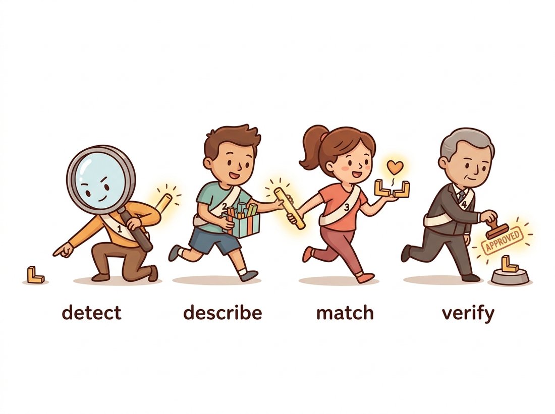
Chapter 9 celebrated edges as the most informative pixels in a single image. The moment a second image enters the picture, the celebration sours. This chapter's opening problem is correspondence: pick a point in image one, find the same physical point in image two. For that job, edges have a fatal flaw, and the first task of this section is to understand the flaw precisely, because the cure is the definition of a corner. The whole chapter is one relay, sketched in the illustration below: detect a point, describe it, match it, then verify the match geometrically.
1. The Correspondence Problem and the Aperture Problem Beginner
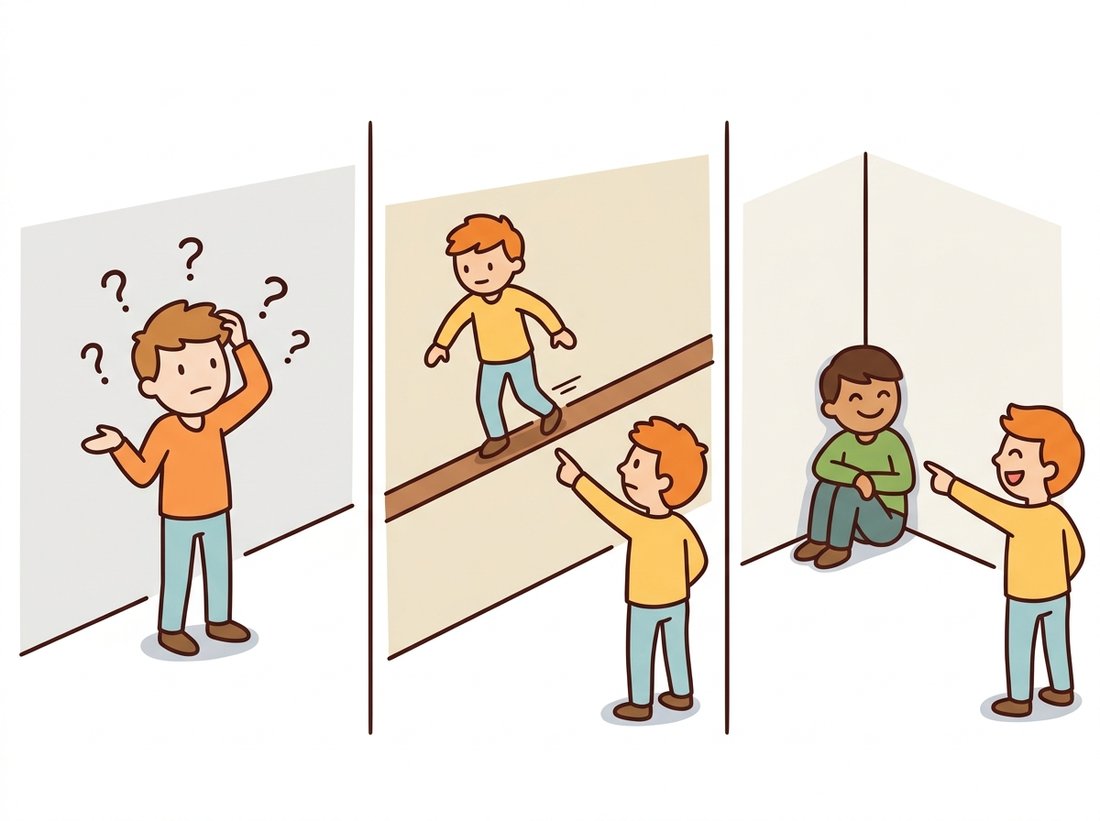
Imagine sliding a small window over a photograph and asking, at each location, a simple question: if I nudge this window a few pixels in any direction, does the patch of pixels inside it change? Three qualitatively different answers exist. Over a blank wall, the patch looks identical no matter where you nudge it; a matcher trying to localize that patch in another image would find thousands of equally good positions. Along an edge, the patch changes when you cross the edge but stays the same when you slide along it; the matcher can pin down one coordinate but not the other. Only at a corner, where two edges meet or texture varies in two directions, does every nudge change the patch. A corner is localizable in both dimensions, and that is the whole reason this chapter hunts for corners rather than edges. The hide-and-seek scene below makes the three cases concrete.
The edge case has a classical name: the aperture problem. Seen through a small aperture, a moving edge appears to move only perpendicular to itself; its motion along its own direction is invisible. The same ambiguity that ruins edge matching here will return in Chapter 15 as the central obstacle of optical flow, and the detectors built in this section are exactly the points where optical flow is well posed. Figure 10.1.1 makes the three-way distinction visual.
Corner detection is not about corners as a shape; it is about selecting the pixels where the correspondence problem has a unique answer. A detector is judged by repeatability: photographed again from a new viewpoint, under new lighting, does it fire at the same physical points? Repeatability, not visual salience, is the metric every detector in this chapter is engineered for. A three-word mnemonic for the structure tensor's verdict captures the whole section: flat ignores, edge slides, corner commits. Flat regions look the same under every shift, edges stay the same when you slide along them, and only corners change under every shift, which is exactly what makes them findable again.
2. The Structure Tensor: Measuring Change in All Directions Intermediate
To turn the sliding-window thought experiment into an algorithm, write it down. Let $I(x, y)$ be a grayscale image and consider shifting a window $W$ by a small offset $(u, v)$. The summed squared difference between the original and shifted patch is
$$ E(u, v) \;=\; \sum_{(x,y) \in W} w(x, y)\, \big[ I(x+u,\, y+v) - I(x, y) \big]^2, $$
where $w$ is a weighting window (Gaussian in practice, so that pixels near the center count more). For small shifts, the first-order Taylor expansion $I(x+u, y+v) \approx I + u\, I_x + v\, I_y$ (the calculus fact that a smooth function near a point is well approximated by its value plus its slope times the step) replaces the image difference with the image gradients $I_x$ and $I_y$, the same quantities the Sobel operator of Chapter 3 computes. Substituting and collecting terms gives a quadratic form
$$ E(u, v) \;\approx\; \begin{bmatrix} u & v \end{bmatrix} M \begin{bmatrix} u \\ v \end{bmatrix}, \qquad M \;=\; \sum_{(x,y) \in W} w(x,y) \begin{bmatrix} I_x^2 & I_x I_y \\ I_x I_y & I_y^2 \end{bmatrix}. $$
The $2 \times 2$ matrix $M$ is the structure tensor (also called the second-moment matrix), and it compresses everything the window knows about local geometry into three numbers. Because $M$ is symmetric, it has two non-negative eigenvalues $\lambda_1 \geq \lambda_2$ with orthogonal eigenvectors, and the quadratic form means exactly this: shifting the window by one pixel along the first eigenvector changes the patch by $\lambda_1$; along the second, by $\lambda_2$. The eigenvalues are the answers to the sliding-window question, measured in the two most informative directions.
The classification follows immediately, and Figure 10.1.2 draws it. If both eigenvalues are small, no shift changes anything: flat. If one is large and the other small, the patch changes only across one direction: edge. If both are large, every shift changes the patch: corner. Note the pleasant continuity with Chapter 9: an edge detector looks for one large gradient direction; a corner detector demands two.
3. The Harris Response Intermediate
In 1988, eigenvalue decompositions were expensive, and Harris and Stephens wanted a corner score for every pixel of every frame. Their trick: you do not need the eigenvalues themselves, only a function that is large when both are large. The determinant and trace of $M$ deliver them indirectly, since $\det M = \lambda_1 \lambda_2$ and $\operatorname{tr} M = \lambda_1 + \lambda_2$, both computable directly from the tensor entries. The Harris response is
$$ R \;=\; \det M - k\,(\operatorname{tr} M)^2 \;=\; \lambda_1 \lambda_2 - k\,(\lambda_1 + \lambda_2)^2, $$
with $k$ an empirical constant, conventionally between 0.04 and 0.06. Work through the three cases: both eigenvalues small gives $R \approx 0$; one large eigenvalue makes the trace term dominate, driving $R$ negative; two large eigenvalues make the determinant win, $R$ large and positive. One formula, three regimes, no eigendecomposition. The purple contour in Figure 10.1.2 shows the resulting decision boundary curving through the eigenvalue plane.
The full detector is the response map plus two cleanup steps: threshold $R$ to keep only confident corners, and apply non-maximum suppression so that each corner contributes one detection rather than a blob of high-response pixels (the same hygiene Canny applied to edges in Chapter 9). The implementation below builds all of it from operations you already own from Chapter 3: two Sobel passes, three Gaussian blurs, and pixelwise arithmetic.
import cv2
import numpy as np

def harris_response(gray: np.ndarray, k: float = 0.05,
                    sigma: float = 1.5) -> np.ndarray:
    """Harris corner response for every pixel, from first principles."""
    g = gray.astype(np.float32) / 255.0
    Ix = cv2.Sobel(g, cv2.CV_32F, 1, 0, ksize=3)    # horizontal gradient
    Iy = cv2.Sobel(g, cv2.CV_32F, 0, 1, ksize=3)    # vertical gradient
    # Structure-tensor entries: products of gradients, Gaussian-windowed
    Sxx = cv2.GaussianBlur(Ix * Ix, (0, 0), sigma)
    Syy = cv2.GaussianBlur(Iy * Iy, (0, 0), sigma)
    Sxy = cv2.GaussianBlur(Ix * Iy, (0, 0), sigma)
    det = Sxx * Syy - Sxy * Sxy                      # lambda1 * lambda2
    trace = Sxx + Syy                                # lambda1 + lambda2
    return det - k * trace * trace

img = cv2.imread("building.jpg", cv2.IMREAD_GRAYSCALE)
R = harris_response(img)

# Keep strong responses that are also the maximum of their 7x7 neighborhood
threshold = 0.01 * R.max()
is_local_max = (R == cv2.dilate(R, np.ones((7, 7), np.uint8)))
ys, xs = np.where((R > threshold) & is_local_max)
print(f"{len(xs)} corners") # typical photo of a building: ~400 cornersThe fifteen-line detector above is one call in OpenCV: R = cv2.cornerHarris(gray, blockSize=2, ksize=3, k=0.05), roughly a 15-to-1 reduction. Internally the library fuses the gradient, windowing, and response arithmetic into a single cache-friendly pass and handles border replication for you. Production pipelines usually add cv2.cornerSubPix, which refines each integer corner to sub-pixel precision by fitting the local gradient field, a refinement camera calibration in Chapter 12 will treat as mandatory rather than optional.
The constant $k$ is the one free knob in the Harris response, and thirty seconds of play teaches more about it than the formula does. Take the harris_response code above and re-run the corner count for $k \in \{0.02, 0.04, 0.06, 0.10\}$, keeping the threshold fixed at 0.01 * R.max(). Watch the count fall as $k$ rises, and overlay the surviving corners on the image each time. Then trace the cause back to the formula $R = \det M - k(\operatorname{tr} M)^2$: a larger $k$ inflates the trace penalty, so points where the two eigenvalues are merely lopsided (near-edges that squeaked in at small $k$) drop below threshold first, while the genuinely two-directional corners hang on. You are watching the decision boundary in Figure 10.1.2 swing toward the corner quadrant.
4. Shi-Tomasi: A Better Score for Trackers Intermediate
Six years after Harris, Shi and Tomasi revisited the response formula while building a feature tracker and proposed something simpler: score each pixel by the smaller eigenvalue alone,
$$ R_{\text{ST}} \;=\; \min(\lambda_1, \lambda_2). $$
The reasoning is beautifully task-driven. A tracker's failure mode is drift along the direction of least information, and that direction's information content is exactly $\lambda_2$. If the worst direction is still strong, the point is trackable; the strength of the best direction is irrelevant once the worst one passes the bar. Geometrically (Figure 10.1.2 again, the teal lines) the acceptance region becomes a clean quadrant: $\min(\lambda_1, \lambda_2) > t$. On modern hardware the eigenvalues of a symmetric $2\times2$ matrix cost a square root, so the historical motivation for avoiding them is gone, and Shi-Tomasi is the default corner scorer in OpenCV's aptly named function:
# Shi-Tomasi detection: keep corners whose smaller eigenvalue is largest,
# spread out by minDistance so detections do not clump on one texture.
corners = cv2.goodFeaturesToTrack(
    img,                  # 8-bit grayscale input
    maxCorners=500,       # cap on detections, strongest first
    qualityLevel=0.01,    # accept corners above 1% of the best score
    minDistance=10,       # spatial spread: no two corners closer than this
    blockSize=3)          # structure-tensor window size
print(corners.shape) # (500, 1, 2): float32 (x, y), ready for trackingcv2.goodFeaturesToTrack: the qualityLevel threshold is relative to the strongest corner found, and minDistance enforces spatial spread so detections do not cluster on the most textured object in the scene.
The minDistance parameter deserves a comment because it encodes a lesson detectors keep re-learning: raw response strength concentrates wherever texture is strongest, but downstream geometry wants coverage. Estimating a homography from 500 corners on one bush and zero on the rest of the frame is numerically legal and practically useless. Spreading detections, whether by minimum distance, per-tile quotas, or adaptive suppression, is standard practice in every serious pipeline, including the SLAM systems of Chapter 14.
The Shi-Tomasi paper is titled "Good Features to Track," which makes it one of the few publications in computer vision whose title is also its API documentation. OpenCV adopted the name verbatim, so thirty years of students have typed a 1994 paper title into their editors, mostly without knowing it.
5. FAST: Corners at Video Rate Intermediate
Harris and Shi-Tomasi compute gradients, products, and blurs for every pixel: a few dozen floating-point operations each. That is nothing for one photograph and a budget-breaker for a robot processing 60 frames per second on an embedded CPU while also doing everything else. FAST (Features from Accelerated Segment Test, Rosten and Drummond, 2006) attacks the cost with a different philosophy: do not measure cornerness, just test for it, as cheaply as possible.
The segment test examines a Bresenham circle of 16 pixels at radius 3 around a candidate pixel $p$ with intensity $I_p$ (a Bresenham circle is just the ring of integer-coordinate pixels that best approximates a circle, so the 16 samples land on actual pixels with no interpolation). The candidate is a corner if at least $n$ contiguous pixels on the circle are all brighter than $I_p + t$ or all darker than $I_p - t$, for a threshold $t$. The standard choice is $n = 9$ (FAST-9), which empirically beats the original $n = 12$ on repeatability. The intuition maps back to Figure 10.1.1: a flat region has no such run, an edge has two runs of about half the circle that are interrupted, and a corner has one long unbroken run of "different" on the outside of the corner.
Two engineering moves make FAST genuinely fast. First, a quick-reject: examine the four compass pixels (top, right, bottom, left); if fewer than three of them are sufficiently brighter or darker, no run of 9 can exist, and most of the image exits after four comparisons. Second, Rosten and Drummond trained a decision tree (classic ID3, on labeled corner data) that orders the remaining pixel tests to maximize information gain, then compiled the tree to branchy code. The detector that results performs a handful of byte comparisons per pixel, no multiplications at all, and runs comfortably at video rate on a microcontroller. The price: FAST returns no cornerness measure of its own, so for non-maximum suppression a score $V$ (the largest $t$ for which the pixel remains a corner) is computed for accepted candidates only.
# FAST segment test: no cornerness math, just count contiguous bright/dark
# pixels on the 16-pixel ring; compare detection counts with and without NMS.
fast = cv2.FastFeatureDetector_create(
    threshold=25,             # intensity margin t for the segment test
    nonmaxSuppression=True,
    type=cv2.FAST_FEATURE_DETECTOR_TYPE_9_16)   # FAST-9 on a 16-pixel circle
kps = fast.detect(img, None)
print(f"with NMS: {len(kps)} keypoints")

fast.setNonmaxSuppression(False)
print(f"without NMS: {len(fast.detect(img, None))} keypoints")
# with NMS: 1247 keypoints
# without NMS: 4108 keypoints (clumps of adjacent detections)Who: A three-engineer perception team at a warehouse-automation startup, running visual odometry on autonomous tugger robots.
Situation: Each robot navigated by tracking features across a downward-tilted camera at 60 fps on a fanless ARM board shared with planning and safety processes. The perception slice of the frame budget was 8 ms, of which detection was allowed 4.
Problem: The prototype used Shi-Tomasi detection at 11 ms per frame on that CPU. It produced beautiful, well-spread corners and missed every deadline. Frames were dropped, odometry drifted, and the robots developed a reputation for gentle but unnerving wall encounters.
Decision: Switch detection to FAST-9 with a fixed threshold, then recover the two Shi-Tomasi properties they actually missed: spread, via an 8x6 grid with a per-cell cap of 12 keypoints; and stability, by keeping the per-corner FAST score and suppressing all but the strongest per cell.
Result: Detection time fell to 0.9 ms per frame, total tracking to 5.6 ms. Odometry drift per 100 meters improved by 22 percent, not because FAST corners were better, but because the system stopped dropping frames. The grid bucketing survived two full hardware generations.
Lesson: Detector quality is a systems property, not a per-keypoint property. A mediocre corner detected every frame beats an excellent corner detected when the CPU happens to be free.
6. Choosing a Detector Beginner
Three detectors, one decision. Table 10.1.1 condenses the trade-offs that the previous sections developed, and one column matters more than the others: none of these detectors survives a change of scale. A corner at one zoom level is a smooth curve at another; the structure tensor and the segment test both operate at a single, fixed neighborhood size. Fixing that is an idea important enough to get its own section, and Section 10.2 builds it.
| Detector | Score | Relative speed | Rotation invariant | Scale invariant | Typical role |
|---|---|---|---|---|---|
| Harris (1988) | $\det M - k(\operatorname{tr} M)^2$ | 1x (baseline) | Yes | No | Accurate corners, calibration targets |
| Shi-Tomasi (1994) | $\min(\lambda_1, \lambda_2)$ | ~1x | Yes | No | Features for tracking (KLT) |
| FAST-9 (2006) | segment test (binary) | 20-40x | Yes (test is radial) | No | Real-time SLAM, basis of ORB |
The table's speed column explains the field's revealed preference: when ORB (Section 10.4) needed a detector to pair with its binary descriptor, it chose FAST and patched its weaknesses (adding a pyramid for scale, an intensity-centroid orientation, and a Harris score for ranking) rather than starting from Harris. Detector and descriptor choices are rarely independent.
The structure tensor asks "does this window change under shift?"; modern research asks a network to learn what is detectable. SuperPoint (2018) made keypoint detection a self-supervised learning problem and remains one of the most widely deployed learned detectors. The 2024 to 2026 wave sharpens both ends of the trade-off this section mapped: XFeat (CVPR 2024) is a learned detector-descriptor explicitly engineered for the CPU-bound niche FAST and ORB occupy, running at hundreds of fps without a GPU; DeDoDe (3DV 2024) decouples detection from description and trains the detector directly on the objective that matters, 3D consistency across views of large reconstruction datasets; and ALIKED (2023) learns deformable, rotation-aware detection. Tellingly, every one of these systems still emits sparse, well-spread, sub-pixel-refined keypoints with non-maximum suppression: the output contract written by Harris in 1988 survived the replacement of everything inside it. The learned-representation story continues in Chapter 25.
For each of the following windows, state (without computing) the approximate eigenvalue pattern of the structure tensor ($\lambda_1$, $\lambda_2$ both small, one large, or both large) and the classification: (a) a window of pure sensor noise on a gray wall, (b) a vertical black-to-white step edge, (c) a 45-degree step edge, (d) the tip of a thin diagonal line two pixels wide, (e) a smooth circular blob much larger than the window. Then explain why case (a) is the dangerous one in practice and which parameter of the Harris pipeline defends against it.
Implement the harris_response function from this section and compare it against cv2.cornerHarris on the same image: normalize both response maps to $[0, 1]$ and report the Pearson correlation and the overlap between their top-200 corners (a match is a pair within 2 pixels). Then sweep $k \in \{0.02, 0.04, 0.06, 0.10\}$ and report how the number of detections above a fixed relative threshold changes. Explain the direction of the change using the formula for $R$.
Measure what this section claimed: detector repeatability. Rotate an image by 15-degree increments using the warping tools of Chapter 5, run Shi-Tomasi and FAST on each rotation, map detections back through the inverse rotation, and count what fraction land within 2 pixels of an original detection. Plot repeatability versus angle for both detectors. Which one degrades at intermediate angles, and what about its sampling geometry explains this?