"Give me four hundred holiday photos in random order, no GPS, no timestamps, and a weekend. I will hand you back a building, the camera that took each picture, and a polite note about the three blurry ones I refused to use."
An Incremental Reconstruction Pipeline, Mildly Smug
Reconstructing 3D from images is not a function call but a pipeline, and a small number of mature open-source tools implement that pipeline end to end so you almost never write it yourself. COLMAP is the reference incremental structure-from-motion (SfM) engine; GLOMAP is its faster global-SfM sibling; OpenMVG plus OpenMVS and AliceVision's Meshroom round out the ecosystem; simultaneous localization and mapping (SLAM) frameworks do the same job in real time; and underneath all of them sit the nonlinear optimizers (Ceres, g2o, GTSAM) that perform the bundle adjustment of Chapter 14. This section is the decision guide.
Section 17.1 handed you the verbs, the single OpenCV calls that detect, match, and triangulate; this section chains those verbs into a pipeline that turns a folder of photos into a 3D model, the second rung of the chapter's verbs-pipelines-scoreboards ladder. Chapter 14 derived the algorithm: detect features, match them across images, estimate relative poses, triangulate points, and refine everything jointly with bundle adjustment. Writing that pipeline from scratch, robustly, for hundreds of unordered images, is a multi-year software project, which is precisely why nobody does it. The community converged on a handful of tools that are correct, fast, and battle-tested. This section maps them, runs the canonical one, and explains the optimization machinery they share, so you can pick the right tool the first time a project needs a 3D model.
1. The Reconstruction Pipeline, and Where the Tools Sit Intermediate
Every photogrammetry tool implements the same conceptual stages, then differs in how it orders and optimizes them. Figure 17.2.1 lays out the canonical flow from images to a textured mesh and marks which tool owns which stage, because the most common architecture in practice is a hybrid: one tool for the sparse reconstruction (the cameras and a point cloud) and another for the dense reconstruction (the surface).
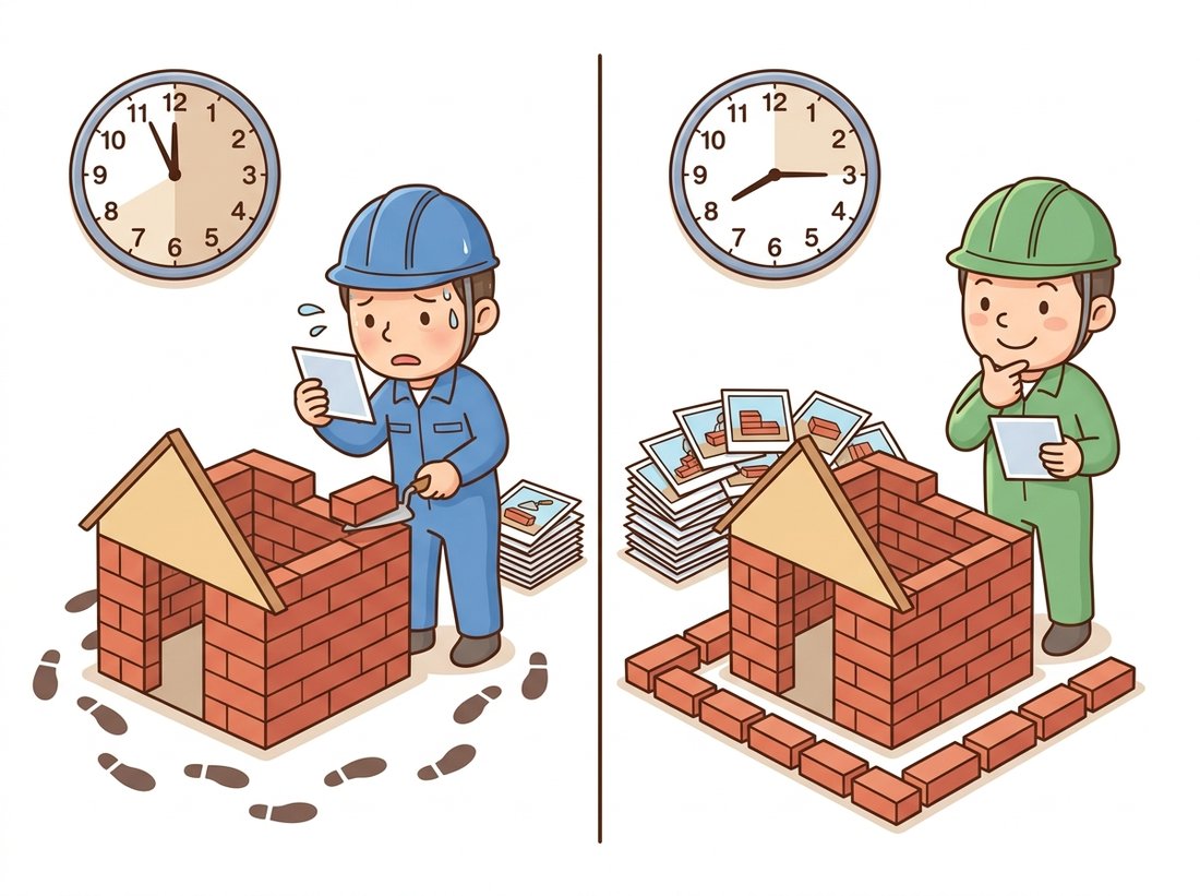
The crucial architectural choice is at the SfM stage: incremental versus global. Incremental SfM (COLMAP) starts from a good two-view pair and adds one image at a time, running bundle adjustment repeatedly; it is extremely robust but scales super-linearly because of the repeated optimization. Global SfM (GLOMAP, OpenMVG's global mode) estimates all camera rotations and translations at once from the pairwise relations, then bundle-adjusts once; it is far faster on large sets but historically more fragile. The 2024 GLOMAP work narrowed that robustness gap considerably, which is why it now appears in the tooling conversation as a serious COLMAP alternative. The illustration below contrasts the two strategies as builders assembling the same house.
The phrase "incremental SfM adds one image at a time, re-running bundle adjustment" sounds linear and cheap. It is neither. Each newly registered image triggers a global refinement over every camera and point seen so far, so the cost of the run grows super-linearly with the image count. The GLOMAP paper makes the gap concrete: on a scene of roughly a thousand internet photos, incremental COLMAP can grind for many hours, while GLOMAP's "solve all rotations and translations at once, then bundle-adjust once" strategy reaches comparable accuracy in minutes, an order-of-magnitude wall-clock difference on the same images and the same final point cloud. That is the whole reason global SfM exists: the two approaches optimize the identical objective, but incremental pays the bundle-adjustment bill once per image while global pays it once per dataset. So when a reconstruction job is measured in coffee breaks instead of seconds, the usual culprit is the matching strategy and the incremental-versus-global choice, not the camera.
2. COLMAP: The Reference Pipeline Intermediate
COLMAP (Schönberger and Frahm, CVPR 2016) is the tool to learn first, because it is the de facto standard: its sparse output format is what neural scene methods in Chapter 27 expect, and its database schema is the interchange format the rest of this section's tools read and write. It offers three ways in: a GUI, a command-line interface, and the pycolmap Python bindings. For a quick result, the automatic_reconstructor wraps the whole pipeline; for control and scripting, pycolmap exposes each stage. Code 17.2.1 runs a full sparse-plus-pose reconstruction from a folder of images in a dozen lines.
# Full sparse reconstruction from a folder of images: extract SIFT
# features into a COLMAP database, match them, then run incremental
# structure-from-motion to recover camera poses and a 3D point cloud.
import pycolmap
from pathlib import Path

image_dir = Path("photos/")
out = Path("reconstruction/"); out.mkdir(exist_ok=True)
db = out / "database.db"

# 1. Detect SIFT features and write them to the COLMAP database.
pycolmap.extract_features(db, image_dir)
# 2. Match features (exhaustive for small sets; use sequential/vocab-tree for large).
pycolmap.match_exhaustive(db)
# 3. Incremental SfM: build the sparse model (cameras + 3D points).
maps = pycolmap.incremental_mapping(db, image_dir, out)

rec = maps[0]                          # the largest reconstructed model
print(f"registered {rec.num_reg_images()} images, "
      f"{rec.num_points3D()} 3D points")
rec.write(out) # cameras.bin, images.bin, points3D.binpycolmap. The three calls map exactly onto the Chapter 14 pipeline: feature extraction, matching, and incremental mapping with bundle adjustment folded into the third call. The output .bin files are the format Chapter 27's NeRF and Gaussian-splatting tools read directly.registered 96 images, 28734 3D points
It is natural to read the points3D coordinates that Code 17.2.1 prints as physical positions, so that a recovered point at $(2.0, 0.0, 5.0)$ sits two units left and five units deep in some real room. From images alone they are nothing of the kind. A structure-from-motion reconstruction from ordinary photographs is fixed only up to a global similarity transform: the entire scene, with all its cameras, can be rotated, translated, and uniformly rescaled without changing a single reprojection, the gauge freedom and monocular scale ambiguity of Chapter 13 and Section 14.3. The coordinates are internally consistent but arbitrary in unit and orientation; doubling them yields an equally valid model. To attach real units you must add metric information the photos do not contain: a known baseline (stereo or a calibrated rig), a measured distance between two points, GPS or inertial data, or an object of known size in the scene. The trap is shipping a reconstruction as if its numbers were meters and discovering in the field, as the localization team in Section 17.3's example did, that nothing holds scale.
The pipeline in Code 17.2.1 is, line for line, the entire structure-from-motion system of Chapter 14: correspondence search, robust two-view initialization, incremental registration via PnP, triangulation, and global bundle adjustment, plus the failure handling for degenerate pairs, drift, and duplicate points that the chapter only sketched. A research-grade implementation of that pipeline is tens of thousands of lines of C++; COLMAP is exactly that codebase, and pycolmap hands it to you in twelve lines of Python. The one judgment call the shortcut still demands is the matching strategy: match_exhaustive is $O(n^2)$ in the image count and only suits sets up to a few hundred images; larger collections need match_sequential (for video) or vocabulary-tree matching (for unordered internet photos).
Code 17.2.1 is already the spine of a portfolio-grade weekend project. Walk around a single object (a shoe, a houseplant, a statue in a park) and shoot 40 to 80 overlapping phone photos with roughly seventy percent overlap between consecutive frames, run the three pycolmap calls to recover the cameras and sparse point cloud, then hand the resulting cameras.bin and images.bin straight to a Gaussian-splatting trainer to get a free-viewpoint 3D model you can spin in a browser. The whole build is a small command-line wrapper plus the eleven lines above; the interesting engineering is the capture discipline (overlap and coverage, exactly the failure mode of this section's Practical Example) and a quality gate that rejects a run when too few images register. The COLMAP output you produce here is the input format the neural scene methods of Chapter 27 consume, so this mini-project is also the on-ramp to Part III's most spectacular results. Difficulty: intermediate; about two to three hours including capture.
The matching strategy is the single biggest lever on both runtime and quality, summarized in Table 17.2.1. Choosing it correctly is the difference between a reconstruction that finishes overnight and one that never finishes.
| Strategy | Cost | Use when |
|---|---|---|
| Exhaustive | $O(n^2)$ pairs | Small unordered set (up to a few hundred images) |
| Sequential | $O(n)$ pairs | Video frames or an ordered capture; matches neighbors in time |
| Vocabulary tree | $O(n \log n)$ | Large unordered collections; retrieves likely overlapping pairs |
| Spatial | $O(n)$ with GPS | Geotagged aerial or street imagery; matches by location |
3. The Ecosystem: GLOMAP, OpenMVG/OpenMVS & Meshroom Intermediate
COLMAP is the default, not the only option, and the alternatives win in specific regimes. Table 17.2.2 is the comparison to keep; the prose below it explains when each tool earns its place.
| Tool | SfM type | Strength | Reach for it when |
|---|---|---|---|
| COLMAP | Incremental | Robust, standard format, huge ecosystem | Default for sparse SfM and Chapter 27 poses |
| GLOMAP | Global | Much faster on large sets, COLMAP-compatible output | Hundreds-to-thousands of images, time matters |
| OpenMVG | Incr. + global | Clean, readable, modular CLI stages | Studying the algorithms or composing custom stages |
| OpenMVS | Dense (MVS) | Best open dense cloud, mesh, texture | You have sparse poses and need a surface |
| Meshroom (AliceVision) | Incremental | GUI node graph, full image-to-mesh | Artists and non-coders; end-to-end with a UI |
GLOMAP (Pan et al., ECCV 2024) is the headline update to the classical toolchain: it performs global SfM that matches incremental COLMAP's accuracy while running an order of magnitude faster on large scenes, and it reads COLMAP's database, so adopting it is a one-binary swap in an existing pipeline. OpenMVG is valued less for raw performance than for clarity: its command-line stages map one-to-one onto the geometry of Chapter 13 and Chapter 14, making it the best codebase to read alongside the theory. The common production pattern is a hybrid: run COLMAP or GLOMAP for the sparse cameras, then hand the result to OpenMVS for the dense point cloud, mesh, and texture. Meshroom, the GUI front-end for AliceVision, wraps an entire pipeline behind a visual node graph and is the tool of choice for artists and anyone who would rather not script.
4. What Runs Underneath: Bundle Adjustment Solvers Advanced
Every tool above shares a beating heart: a nonlinear least-squares solver that performs bundle adjustment, the joint refinement of all camera poses and all 3D points to minimize total reprojection error. From Chapter 14, the objective is
$$ \min_{\{C_j\},\,\{X_i\}} \; \sum_{i,j} v_{ij} \, \rho\!\left( \left\lVert \pi(C_j, X_i) - x_{ij} \right\rVert^2 \right), $$
where $\pi$ projects 3D point $X_i$ through camera $C_j$, $x_{ij}$ is the observed image point, $v_{ij}$ flags whether point $i$ is visible in image $j$, and $\rho$ is a robust loss (Huber or Cauchy) that prevents a few mismatched correspondences from dominating the fit.
This is a giant sparse problem, and the sparsity is the only reason it is solvable: a typical reconstruction has thousands of cameras but a single 3D point is seen by perhaps a handful of them, so $v_{ij}$ is well over 99 percent zeros. A naive dense solver would choke on the millions-by-millions normal-equation matrix; the solvers here exploit that emptiness, factoring only the few nonzero blocks, which is what turns an impossibly large optimization into one that finishes on a laptop. The mental model below makes that emptiness concrete. Three libraries dominate, and which one a tool uses tells you something about its design, as Table 17.2.3 shows.
Think of the visibility relationship as a wedding seating chart rather than a round-robin tournament. A round-robin would pair every camera with every 3D point, the dense millions-by-millions matrix a naive solver tries to build. But a 3D point is like a guest who only knows the handful of people at their own table: each point is seen by a few cameras, never by all of them. The seating chart records only those few real acquaintances and leaves the rest of the grid blank, so writing down "who knows whom" costs a few entries per guest instead of one entry per pair of guests. The sparse solver reads exactly that chart: it does arithmetic only where a camera and a point actually share an observation (the nonzero blocks of $v_{ij}$) and skips the vast empty remainder, which is why the cost scales with the real observations rather than with cameras times points.
Where this model breaks down: a seating chart is fixed, but bundle adjustment re-reads the same sparsity pattern every iteration and a few densely-observed points (a landmark seen from almost everywhere) still create heavy rows that dominate the solve.
| Solver | Model | Used by | Character |
|---|---|---|---|
| Ceres Solver | General nonlinear least squares | COLMAP, GLOMAP | Auto-diff, flexible cost functions, batch SfM |
| g2o | Graph optimization | ORB-SLAM2/3 | Hyper-graph of poses and landmarks, real-time |
| GTSAM | Factor graphs (iSAM) | Many SLAM back-ends | Incremental smoothing, marginalization, inertial (IMU) factors |
You rarely call these directly, but knowing they exist demystifies the tools. Ceres (Agarwal, Mierle et al.) is a general-purpose solver with automatic differentiation, so COLMAP can express the projection cost in plain C++ and let Ceres compute derivatives; it is the batch-SfM workhorse. g2o models the problem as a graph of pose and landmark vertices joined by measurement edges and is tuned for the real-time loop of ORB-SLAM3 (Campos et al., IEEE T-RO 2021). GTSAM uses factor graphs and incremental smoothing (iSAM2) to update a solution as new measurements arrive without re-solving from scratch, which is why it underpins many SLAM and visual-inertial back-ends.
COLMAP and ORB-SLAM3 look like different worlds, one is a batch tool you run on a photo folder, the other a real-time system on a robot, but they solve the identical optimization: minimize reprojection error over poses and points. The difference is the budget. Offline SfM can afford repeated global bundle adjustment over every image, so it chooses Ceres and incremental registration. SLAM must answer in milliseconds per frame, so it optimizes a sliding window of recent keyframes (g2o or GTSAM), keeps a separate slow loop-closure thread to correct drift, and accepts a slightly less accurate map in exchange for keeping up with the camera. Understanding that they share an objective means a debugging instinct from one transfers directly to the other. The phrase to keep: SLAM is bundle adjustment on a deadline.
COLMAP's reach quietly outgrew its paper. Released in 2016 as a structure-from-motion tool, it has since become the unglamorous first step of nearly every shiny 3D result you have seen: the radiance fields of Chapter 27 need camera poses, and the field reached such consensus that "poses from COLMAP" appears in the methods section of thousands of NeRF and Gaussian-splatting papers, usually in a single sentence that hides several CPU-hours of bundle adjustment. A 2016 classical-geometry tool is the silent prerequisite of the 2026 generative-3D boom. The most-cited line in modern 3D is one nobody bothers to write out in full.
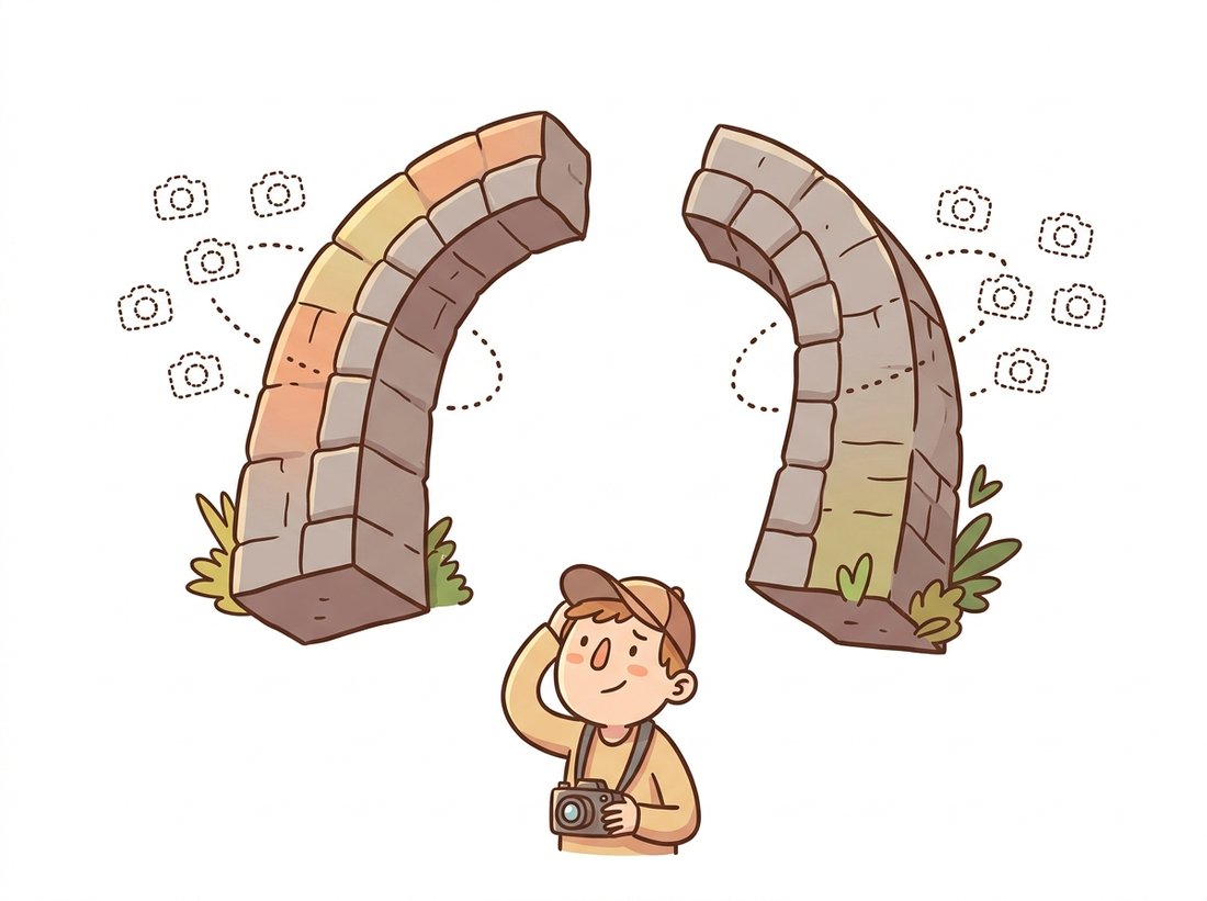
Who: A heritage-preservation group digitizing a stone archway from a phone-camera walkaround.
Situation: They captured 220 images circling the arch and ran COLMAP with exhaustive matching, expecting one clean model.
Problem: COLMAP returned two disconnected reconstructions, the front face and the back face, each internally consistent but with no shared cameras. The arch's two sides had almost no overlapping views, so no feature matches bridged them, and incremental SfM had no way to know the two halves belonged together. The illustration below shows the failure: with no overlapping views to bridge them, the arch reconstructs as two floating halves.
Dilemma: They weighed three responses. They could force the two models together by hand-aligning them in a mesh editor, fast but geometrically unjustified and certain to introduce seams. They could re-shoot the entire 220-image sequence with a denser orbit, the safest fix but a half-day return trip to the site. Or they could capture only a short bridging sequence over the gap and re-match, cheap and targeted but dependent on getting the bridge coverage right the first time.
Decision: Instead of fighting the matcher, they shot a short connecting sequence of images sweeping around one edge of the arch, then re-ran with sequential matching enabled on that bridge so the two halves shared correspondences. They also enabled loop-closure-style re-matching of geometrically verified pairs.
Result: The next run produced a single connected model registering 214 of 220 images. The six dropped images were genuinely blurry, and COLMAP's refusal to register them was correct behavior, not a bug.
Lesson: Disconnected reconstructions are a coverage problem, not a software failure. SfM can only connect what shares features; plan the capture so that consecutive views overlap by roughly sixty to eighty percent and that loops close. The tool is honest about what it cannot see.
The 2024 to 2025 frontier collapses the multi-stage pipeline of Figure 17.2.1 into a single neural network forward pass. DUSt3R (Wang et al., CVPR 2024) regresses a dense, aligned 3D point map directly from an uncalibrated image pair, skipping explicit matching and SfM entirely, and its successor MASt3R adds metric scale and a matching head. VGGT (Wang et al., CVPR 2025) pushes this to many images at once, predicting cameras, depth, and 3D points for a whole set in seconds where COLMAP would take minutes to hours. In parallel, the classical pipeline is being upgraded rather than replaced: the hloc toolbox (Sarlin et al.) swaps SuperPoint and LightGlue into COLMAP's front-end, and GLOMAP modernizes the back-end. The honest 2026 picture: feed-forward models win on speed and on hard sparse-view cases, while COLMAP-class pipelines still win on large, high-accuracy reconstructions and remain the trusted ground truth that the learned methods are benchmarked against. The feed-forward methods reappear as first-class tools in Chapter 27.
For each scenario, name the tool or tool combination from Table 17.2.2 you would reach for and justify it in one sentence: (a) recovering camera poses for a 60-image NeRF capture; (b) reconstructing a textured mesh of a sculpture for a museum web viewer, by a curator who does not code; (c) building a sparse model from 3,000 crowd-sourced photos of a landmark, overnight; (d) studying exactly how global rotation averaging works by reading source code.
Capture or download 30 to 80 overlapping images of a small object. Run the Code 17.2.1 pycolmap pipeline. Then load the result and report: how many images registered versus how many you provided, the number of 3D points, and the mean reprojection error (rec.compute_mean_reprojection_error()). Re-run with match_sequential instead of match_exhaustive and compare registered-image counts and runtime. Explain the difference in terms of Table 17.2.1.
The bundle-adjustment objective uses a robust loss $\rho$ rather than plain squared error. Consider a reconstruction with 10,000 correspondences, of which 50 are gross mismatches with reprojection errors of 200 pixels while the rest sit near 1 pixel. Estimate how much a single gross outlier contributes to the total cost under squared loss versus under a Huber loss with threshold 4 pixels. Argue quantitatively why removing $\rho$ would let the 50 outliers bend the entire camera solution, connecting this to the RANSAC pre-filtering of Chapter 13.