ResNet: Residual Learning Changes Everything

"They asked me to learn a function. I said: let me learn only the part you got wrong, and pass the rest along untouched. Suddenly I was a hundred layers deep and still standing."

A Residual Block With Excellent Posture

At the end of Section 20.2 we framed depth and width as a tradeoff and warned that plain depth eventually stops helping. ResNet, from Kaiming He and colleagues at Microsoft Research in 2015, identified precisely why and removed the obstacle. The result was so decisive that it won every major recognition track that year and became the default backbone for the better part of a decade. This section explains the bottleneck (degradation), the fix (residual learning), why the fix works (gradient flow), and the engineering form you will actually use (the bottleneck block).

1. The Degradation Problem Intermediate

Here is the puzzle that motivated ResNet. Take a working network and add more layers. Intuitively, the deeper network should do at least as well as the shallower one, because the extra layers could in principle learn the identity function and simply pass their input through unchanged, leaving accuracy unharmed. Yet the He team observed the opposite: a 56-layer plain network had higher training error than a 20-layer one. This is not overfitting, where training error is low but test error is high; the training error itself was worse. The deeper network was failing to learn even on data it had seen. They named this the degradation problem, pictured in the illustration below as a tall tower of stacked blocks that buckles under its own depth.

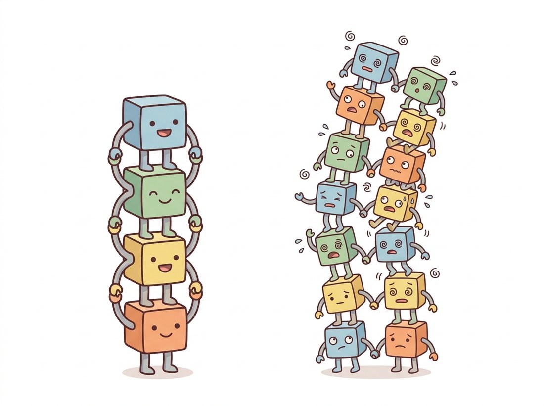
The diagnosis is subtle. The optimizer struggles to make a stack of nonlinear layers represent the identity. Pushing $\text{ReLU}(W_2 \cdot \text{ReLU}(W_1 x + b_1) + b_2)$ to equal $x$ requires a precise and awkward setting of the weights, and gradient descent does not find it easily. So the very capacity that should have been harmless, the ability to do nothing, is hard to learn, and the extra layers actively hurt. Figure 20.3.1 contrasts the failing plain block with the residual fix.

2. The Residual Connection Intermediate

The fix reframes what each block is asked to learn. Instead of asking a block to produce the desired output $H(x)$ directly, ask it to produce the residual $F(x) = H(x) - x$, and recover the output by adding the input back:

The term $+x$ is the identity shortcut (or skip connection): the input is carried forward, unchanged, by simple addition. Now learning the identity mapping is trivial, the optimizer just drives the weights of $F$ toward zero, which is easy. More generally, if the optimal function is close to the identity (as it often is once a network is deep enough), the block only has to learn a small perturbation, which is a far gentler optimization problem than learning the full mapping from scratch. The degradation problem evaporates: a residual network with hundreds of layers trains with lower error than its shallower counterpart, exactly the monotone improvement the plain network failed to deliver.

The code below turns that one-line idea into the building unit you will actually stack, the ResNet basic block: two convolutions, then the input added back.

# The ResNet basic block: two 3x3 conv-BN layers whose output is added back
# to the input. A 1x1 projection shortcut only appears when the block changes
# spatial size or channel count, so the addition always has matching shapes.
import torch
import torch.nn as nn
import torch.nn.functional as F

class BasicBlock(nn.Module):
    """The ResNet basic block (used in ResNet-18 and ResNet-34)."""
    def __init__(self, in_ch, out_ch, stride=1):
        super().__init__()
        self.conv1 = nn.Conv2d(in_ch, out_ch, 3, stride=stride, padding=1, bias=False)
        self.bn1 = nn.BatchNorm2d(out_ch)
        self.conv2 = nn.Conv2d(out_ch, out_ch, 3, padding=1, bias=False)
        self.bn2 = nn.BatchNorm2d(out_ch)
        # Projection shortcut only when shape changes (stride > 1 or channels differ):
        self.shortcut = nn.Sequential()
        if stride != 1 or in_ch != out_ch:
            self.shortcut = nn.Sequential(
                nn.Conv2d(in_ch, out_ch, 1, stride=stride, bias=False),  # 1x1 match shape
                nn.BatchNorm2d(out_ch))

    def forward(self, x):
        out = F.relu(self.bn1(self.conv1(x)))
        out = self.bn2(self.conv2(out))
        out = out + self.shortcut(x)   # the residual addition: F(x) + x
        return F.relu(out)             # ReLU AFTER the add, per the original design

block = BasicBlock(64, 128, stride=2)
print(block(torch.randn(1, 64, 56, 56)).shape)

Two engineering details in the code matter. First, when a block changes the spatial size (stride $> 1$) or the channel count, the identity $x$ no longer matches the shape of $F(x)$, so a $1 \times 1$ convolution (the channel mixer of Section 20.2) projects the shortcut to the right shape. Second, the ReLU is applied after the addition, so the skip path itself is a clean, unactivated identity. Both choices keep the shortcut as close to a pure identity as possible, which is what preserves gradient flow.

3. Why It Works: Gradients Take the Highway Advanced

The deeper reason the residual connection helps is what it does to the backward pass. Recall from Chapter 18 that backpropagation multiplies gradients layer by layer, and that long products of small numbers vanish toward zero. Consider the gradient of the loss $L$ with respect to a block's input $x$ when $y = F(x) + x$. By the chain rule:

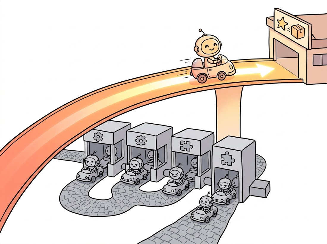
The crucial term is the $+1$. Even if $\partial F / \partial x$ becomes tiny, the gradient flowing back to $x$ is at least $\partial L / \partial y$ itself, carried by the identity path. Stack many residual blocks and the loss gradient reaches the earliest layers essentially undiminished, traveling along the skip connections as if on a highway, while the convolutional branches add their corrections. This is the same mechanism that the residual stream of the transformer relies on, and it is why both architectures can be made extremely deep. The skip connection does not just help; it changes the optimization landscape into one gradient descent can navigate. The illustration below renders that highway literally.

4. The Bottleneck Block and the ResNet Family Intermediate

For the deeper variants (ResNet-50, ResNet-101, ResNet-152), the basic two-convolution block becomes too expensive, so ResNet introduces the bottleneck block: a $1 \times 1$ convolution squeezes the channels down, a $3 \times 3$ convolution does the spatial work on the cheaper narrow representation, and a $1 \times 1$ convolution expands the channels back up. The $3 \times 3$ layer, the expensive one, now operates on one quarter of the channels, and the two $1 \times 1$ layers reshape cheaply, another reuse of the $1 \times 1$ bottleneck from Inception. The full ResNet is then a stem (a $7 \times 7$ convolution and a max-pool), four stages of these blocks at increasing channel counts, global average pooling, and a single linear classifier, the parameter-light head GoogLeNet pioneered.

# The deep-ResNet bottleneck block factors the work into three steps: a 1x1
# squeeze of the channels, a 3x3 spatial conv on the cheap narrow tensor, and
# a 1x1 expand back up by 4x. The residual addition closes the block as before.
import torch.nn as nn
import torch.nn.functional as F

class Bottleneck(nn.Module):
    """ResNet bottleneck: 1x1 squeeze -> 3x3 spatial -> 1x1 expand (4x)."""
    expansion = 4
    def __init__(self, in_ch, mid_ch, stride=1):
        super().__init__()
        out_ch = mid_ch * self.expansion
        self.conv1 = nn.Conv2d(in_ch, mid_ch, 1, bias=False)            # squeeze
        self.bn1 = nn.BatchNorm2d(mid_ch)
        self.conv2 = nn.Conv2d(mid_ch, mid_ch, 3, stride=stride,
                               padding=1, bias=False)                   # spatial
        self.bn2 = nn.BatchNorm2d(mid_ch)
        self.conv3 = nn.Conv2d(mid_ch, out_ch, 1, bias=False)           # expand
        self.bn3 = nn.BatchNorm2d(out_ch)
        self.shortcut = nn.Sequential()
        if stride != 1 or in_ch != out_ch:
            self.shortcut = nn.Sequential(
                nn.Conv2d(in_ch, out_ch, 1, stride=stride, bias=False),
                nn.BatchNorm2d(out_ch))

    def forward(self, x):
        out = F.relu(self.bn1(self.conv1(x)))
        out = F.relu(self.bn2(self.conv2(out)))
        out = self.bn3(self.conv3(out))
        return F.relu(out + self.shortcut(x))

# A ResNet-50 stacks [3, 4, 6, 3] of these blocks across four stages.
print("expansion factor:", Bottleneck.expansion)

# Load a full pretrained ResNet-50 with one call, two ways. The torchvision
# IMAGENET1K_V2 weights bake in the modern training recipe; timm's num_classes
# swaps the 1000-class head for your own label count in the same line.
from torchvision.models import resnet50, ResNet50_Weights
model = resnet50(weights=ResNet50_Weights.IMAGENET1K_V2).eval()  # 80.9% top-1
# Or via timm, with hundreds of ResNet variants and recipes:
import timm
model = timm.create_model("resnet50", pretrained=True, num_classes=10)  # re-headed