Semantic Segmentation: FCN, U-Net & DeepLab

"A classifier squints at the whole picture and shouts one word. I was asked to whisper a word to every pixel, and to make the whispers agree along the edges. The hard part was never the whispering; it was remembering, after all that pooling, where the edges had been."

A Decoder Trying to Undo the Encoder's Forgetting

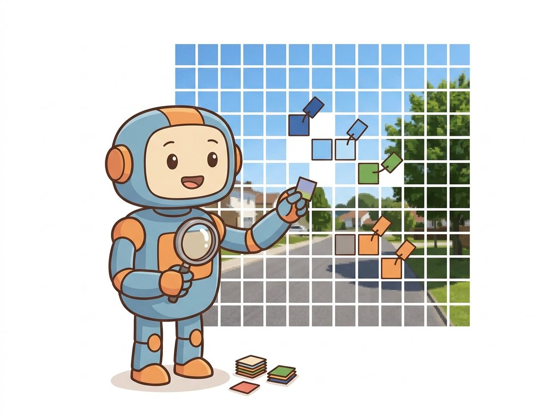
In Chapter 23 a network learned to localize objects with boxes; a box is a rectangle, and the world is not made of rectangles. Semantic segmentation asks the finest spatial question we can pose to a vision model: for every pixel, what category does it belong to? The output is no longer a single label or a handful of boxes but a full-resolution map the same size as the input, where each location holds a class index. There is no notion of separate objects yet, two adjacent cars become one connected blob of the "car" class, that is the job of Section 24.2. Here the question is purely "what," answered everywhere at once (the illustration below makes the contrast with whole-image classification concrete).

1. The Task and the Resolution Problem Beginner

Take any image classifier from Chapter 20, say a ResNet. It alternates convolutions with downsampling so that a $224 \times 224$ input becomes a $7 \times 7$ grid of deep feature vectors before a global pool and a linear layer produce one label. That downsampling is not incidental; it is how the receptive field grows large enough to recognize whole objects, and it is how the network stays affordable. But a segmenter needs an output the size of the input, and a $7 \times 7$ map cannot localize a thin road sign or a hair-thin boundary. This is the resolution problem, and it has a precise shape: deep features are semantically rich but spatially coarse, while shallow features are spatially precise but semantically shallow. Good segmentation needs both.

The first move, due to the fully convolutional network (FCN) of Long, Shelhamer, and Darrell in 2015, is almost embarrassingly simple. A classifier's final layers are fully connected, which forces a fixed input size and discards spatial layout. Replace each of them with an equivalent $1 \times 1$ convolution, and the network becomes "fully convolutional": it accepts any input size and produces a coarse spatial map of class scores instead of one vector. Upsample that coarse map back to the input resolution and you have a segmentation, blurry, but a segmentation. The genuine contribution was fixing the blur, and Figure 24.1.1 shows how.

The skip connections are the heart of FCN. The coarse prediction from the deepest layer (stride 32) knows what is in the scene but not precisely where. So FCN upsamples it by 2 and adds the prediction computed from the stride-16 feature map, then upsamples again and adds the stride-8 prediction. Each addition injects spatial detail the deep layer had thrown away. The result, called FCN-8s, has the semantics of the deep layers and boundaries sharp enough to be useful. This pattern, fuse a coarse-but-deep map with a fine-but-shallow one, is the same multi-scale idea you met as the Gaussian and Laplacian pyramids of Chapter 4, now learned instead of hand-built.

2. U-Net: Symmetric Encoder-Decoder Beginner

U-Net, published the same year as FCN for biomedical images, took the skip idea to its logical conclusion and became the most widely used segmentation architecture ever written. Its shape is a U: a contracting encoder that halves resolution and doubles channels stage by stage, then an expanding decoder that mirrors the encoder, doubling resolution and halving channels. The crucial detail is that at every decoder stage, the upsampled feature map is concatenated with the encoder feature map of the same resolution before further convolution. Where FCN added a few coarse skips, U-Net wires a skip at every level, so detail is reinjected continuously, not just at the end. The illustration below offers a mental model for that continuous reinjection, and Figure 24.1.2 shows the symmetry.

The code below implements a compact U-Net. Read it against Figure 24.1.2: DoubleConv is the two-convolution block at each level (each convolution followed by the batch normalization of Section 19.4, which rescales activations to stabilize training, and a ReLU), the encoder stores its outputs in skips, and each decoder stage upsamples and concatenates the matching skip before convolving. This is a complete, trainable model.

# A compact, fully trainable U-Net for semantic segmentation.
# DoubleConv is the per-level two-conv block; the encoder stores its outputs
# as skips, and each decoder stage upsamples then concatenates the matching skip.
import torch
import torch.nn as nn
import torch.nn.functional as F

class DoubleConv(nn.Module):
    """Two 3x3 convs, each followed by BatchNorm and ReLU. The U-Net building block."""
    def __init__(self, in_ch, out_ch):
        super().__init__()
        self.block = nn.Sequential(
            nn.Conv2d(in_ch, out_ch, 3, padding=1, bias=False),
            nn.BatchNorm2d(out_ch), nn.ReLU(inplace=True),
            nn.Conv2d(out_ch, out_ch, 3, padding=1, bias=False),
            nn.BatchNorm2d(out_ch), nn.ReLU(inplace=True),
        )
    def forward(self, x):
        return self.block(x)

class UNet(nn.Module):
    def __init__(self, in_ch=3, num_classes=21, widths=(64, 128, 256, 512)):
        super().__init__()
        self.downs = nn.ModuleList()
        self.ups = nn.ModuleList()
        self.pool = nn.MaxPool2d(2)
        prev = in_ch
        for w in widths:                       # build the contracting path
            self.downs.append(DoubleConv(prev, w))
            prev = w
        self.bottleneck = DoubleConv(widths[-1], widths[-1] * 2)
        for w in reversed(widths):             # build the expanding path
            self.ups.append(nn.ConvTranspose2d(w * 2, w, 2, stride=2))  # learnable upsample
            self.ups.append(DoubleConv(w * 2, w))   # in_ch = w (up) + w (skip)
        self.head = nn.Conv2d(widths[0], num_classes, 1)   # 1x1 -> per-pixel logits

    def forward(self, x):
        skips = []
        for down in self.downs:
            x = down(x)
            skips.append(x)                    # save full-resolution features
            x = self.pool(x)
        x = self.bottleneck(x)
        skips = skips[::-1]                     # deepest skip first
        for i in range(0, len(self.ups), 2):
            x = self.ups[i](x)                  # transposed conv: upsample
            skip = skips[i // 2]
            if x.shape[-2:] != skip.shape[-2:]: # guard odd sizes
                x = F.interpolate(x, size=skip.shape[-2:], mode="nearest")
            x = torch.cat([skip, x], dim=1)     # concatenate the skip
            x = self.ups[i + 1](x)              # fuse with a DoubleConv
        return self.head(x)                     # (B, num_classes, H, W)

model = UNet(num_classes=21)
logits = model(torch.randn(2, 3, 256, 256))
print(logits.shape)       # torch.Size([2, 21, 256, 256])

The output shape, (2, 21, 256, 256), is the whole point: a 21-class logit vector at each of the $256 \times 256$ pixels of each of the 2 images in the batch. To train it, you pass these logits and an integer label map of shape (2, 256, 256) to nn.CrossEntropyLoss, which treats every pixel as an independent classification example. The transposed convolution (ConvTranspose2d) is a learnable upsampler; we will compare it with simple interpolation and with the dilated approach next.

3. DeepLab: Dilated Convolutions and Atrous Spatial Pyramid Pooling Intermediate

FCN and U-Net both let the backbone shrink the feature map and then fight to rebuild it. DeepLab questions the premise: why lose the resolution at all? The trick is the dilated (also called atrous) convolution, which inserts gaps between the kernel taps. Picture looking at a wide scene through a set of window blinds: you keep the same nine eyes (the nine weights of a $3 \times 3$ kernel), but by spreading them out across the slats you take in a far wider view than if they were clustered together, all without growing a single extra eye. A standard $3 \times 3$ kernel with dilation rate $r$ samples the input at positions spaced $r$ apart, so its receptive field grows from $3$ to $1 + 2r$ in each dimension while the number of weights, and the output resolution, stay the same. Where the blinds analogy breaks down: real blinds simply block the slats in between, whereas a dilated convolution skips those positions for this one layer but stacking several dilated layers eventually covers them, so no input pixel is permanently ignored. Set $r = 2$ and a $3 \times 3$ kernel covers a $5 \times 5$ region; set $r = 4$ and it covers $9 \times 9$. You enlarge the receptive field, the thing that downsampling was buying you, without ever downsampling. Figure 24.1.3 shows the same nine taps spreading across the grid as the dilation rate climbs.

The output size of a convolution with kernel $k$, dilation $r$, padding $p$, and stride $s$ on an input of size $n$ is

With the effective kernel size $k_{\text{eff}} = r(k-1) + 1$ standing in for $k$, this is just the ordinary convolution-size formula from Chapter 19. Stride $N$ simply means the feature map is $N$ times smaller than the input, so a smaller stride means a larger, more detailed map. DeepLab keeps the backbone's late stages at stride 8 or 16 instead of 32, replacing the lost stride with dilation so the receptive field still reaches whole objects. On top of the high-resolution feature map it places atrous spatial pyramid pooling (ASPP): several parallel dilated convolutions at different rates, plus a global pooling branch, all concatenated. Because each branch sees a different effective scale, ASPP captures objects from small to large in one shot, the learned analog of running a detector over an image pyramid. The code below shows dilation in action and a minimal ASPP.

# Dilation in action, then a minimal ASPP module.
# The dilated conv enlarges the receptive field without shrinking the map;
# ASPP runs several dilation rates plus global pooling in parallel and fuses them.
import torch
import torch.nn as nn

# A dilated 3x3 conv keeps spatial size but enlarges the receptive field.
x = torch.randn(1, 64, 64, 64)
plain   = nn.Conv2d(64, 64, 3, padding=1, dilation=1)  # RF 3x3, out 64x64
dilated = nn.Conv2d(64, 64, 3, padding=4, dilation=4)  # RF 9x9, out 64x64
print(plain(x).shape, dilated(x).shape)   # both torch.Size([1, 64, 64, 64])

class ASPP(nn.Module):
    """Atrous Spatial Pyramid Pooling: parallel dilated convs + image-level pooling."""
    def __init__(self, in_ch, out_ch=256, rates=(6, 12, 18)):
        super().__init__()
        self.branches = nn.ModuleList(
            [nn.Conv2d(in_ch, out_ch, 1)] +                       # 1x1 branch
            [nn.Conv2d(in_ch, out_ch, 3, padding=r, dilation=r)   # dilated branches
             for r in rates]
        )
        self.pool = nn.Sequential(nn.AdaptiveAvgPool2d(1),        # global context
                                  nn.Conv2d(in_ch, out_ch, 1))
        self.project = nn.Conv2d(out_ch * (len(rates) + 2), out_ch, 1)

    def forward(self, x):
        feats = [b(x) for b in self.branches]
        g = self.pool(x)
        g = nn.functional.interpolate(g, size=x.shape[-2:], mode="bilinear",
                                      align_corners=False)         # broadcast to map size
        feats.append(g)
        return self.project(torch.cat(feats, dim=1))

print(ASPP(64)(x).shape)   # torch.Size([1, 256, 64, 64])

DeepLabv3+ then adds a small decoder, a single U-Net-style skip from an early high-resolution layer, to sharpen boundaries that even the dilated features leave a little soft. So the three architectures converge: FCN fuses a few skips, U-Net fuses skips everywhere, and DeepLab avoids most of the loss then fuses one skip to clean up. All three are answering the same resolution problem stated in subsection 1.

4. Training and Inference in Practice Intermediate

At inference, the network produces logits of shape (B, C, H, W), and the predicted label map is simply the argmax over the class dimension. The thresholding-and-argmax step is the dense version of the thresholding you met in Chapter 2 and the per-pixel decision that morphology in Chapter 6 then cleans up. The training loss, as established in subsection 2, is a per-pixel cross-entropy; the full menu of losses for imbalanced and boundary-heavy cases is the subject of Section 24.6. The short training and inference loop below ties the model from subsection 2 to real tensors.

# One end-to-end dense-prediction loop: a single training step then inference.
# CrossEntropyLoss treats every pixel as an independent classification example;
# argmax over the class channel turns the logit map into a predicted label map.
import torch, torch.nn as nn

model = UNet(num_classes=21)                       # from subsection 2
criterion = nn.CrossEntropyLoss(ignore_index=255)  # 255 = "unlabeled", skipped in the loss
optimizer = torch.optim.AdamW(model.parameters(), lr=1e-3)

# One training step on a dummy batch.
images = torch.randn(4, 3, 256, 256)               # (B, 3, H, W)
targets = torch.randint(0, 21, (4, 256, 256))      # (B, H, W) integer class per pixel
logits = model(images)                             # (B, 21, H, W)
loss = criterion(logits, targets)                  # per-pixel cross-entropy, auto-averaged
loss.backward(); optimizer.step(); optimizer.zero_grad()
print(f"loss: {loss.item():.3f}")                  # e.g. loss: 3.085

# Inference: argmax over the class channel gives the predicted label map.
model.eval()
with torch.no_grad():
    pred = model(images).argmax(dim=1)             # (B, H, W) predicted classes
print(pred.shape, pred.unique().numel(), "classes present")

# Load a COCO-pretrained DeepLabv3 and run it in four lines.
# weights.transforms() supplies the exact preprocessing the model was trained with,
# so we never hand-write resize-and-normalize; argmax turns logits into a mask.
import torch
from torchvision.models.segmentation import deeplabv3_resnet50, DeepLabV3_ResNet50_Weights

weights = DeepLabV3_ResNet50_Weights.DEFAULT
model = deeplabv3_resnet50(weights=weights).eval()   # backbone + ASPP + classifier
preprocess = weights.transforms()                    # resize, normalize, to-tensor

img = torch.rand(3, 520, 520)                         # stand-in for a loaded PIL image tensor
batch = preprocess(img).unsqueeze(0)
with torch.no_grad():
    out = model(batch)["out"]                         # (1, 21, H, W) logits
mask = out.argmax(1)[0]                               # predicted label map
print(mask.shape)                                     # torch.Size([520, 520])