Action Recognition: 3D CNNs & Two-Stream Networks

"You taught me to slide a little window over an image and call what I found an edge. So I slid a little box over a stack of images, and what I found was a wave goodbye. Same trick, one more dimension, infinitely more drama."

A 3D Convolution Kernel With a Flair for the Theatrical

In Section 26.1 we turned a video into a clip tensor of shape $(C, T, H, W)$. Now we feed that tensor to a network that must output an action label. The chapter's central question, where to spend compute between the spatial and temporal axes, gets its first two concrete answers here. We start with the 3D convolution, see why it works and why it is costly, then study the orthogonal two-stream design that splits the problem in half. Both predate the video transformers of Section 26.3, but neither is obsolete; the factorized 3D blocks and the SlowFast multi-rate idea remain in production systems and inform transformer design.

1. The 3D Convolution Beginner

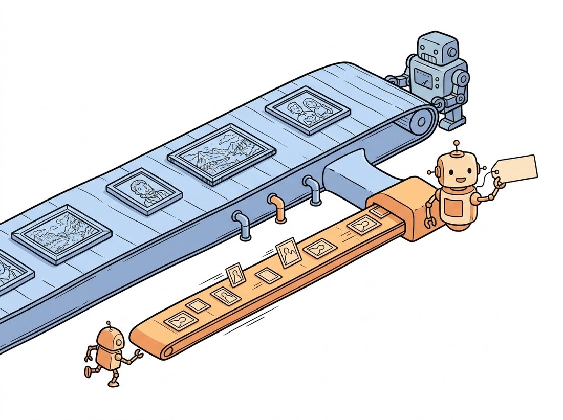
Recall the 2D convolution: a kernel of shape $(C_{in}, k_h, k_w)$ slides over the height and width of an image, and at each position it computes a dot product, producing one output value per spatial location per output channel. A 3D convolution does the identical thing with one more axis. Its kernel has shape $(C_{in}, k_t, k_h, k_w)$, and it slides over time as well as height and width. Where a 2D kernel sees a small spatial patch, a 3D kernel sees a small spatiotemporal cube: a patch of the image across several consecutive frames. A kernel that responds to a bright region moving rightward across three frames is detecting rightward motion, exactly as a Sobel kernel from Chapter 3 detects a vertical edge, and just as in the 2D case those kernels are learned, not designed. The illustration below shows how spanning several frames at once turns a spatial edge into motion.

The output of a 3D convolution is itself a 4D feature map $(C_{out}, T', H', W')$, so 3D convolutions stack exactly like 2D ones, building a hierarchy of increasingly abstract spatiotemporal features. The cost of the generalization is multiplicative. A 2D kernel has $C_{in} \cdot k_h \cdot k_w$ weights per output channel; the 3D version multiplies that by $k_t$, and the number of output positions is also multiplied by the temporal extent. For a typical $3 \times 3 \times 3$ kernel this is a $3\times$ increase in parameters and a substantial increase in compute and activation memory over the 2D equivalent. Figure 26.2.1 contrasts the two operations.

The PyTorch implementation needs only the 3D versions of the layers you already know. nn.Conv3d, nn.BatchNorm3d, and nn.MaxPool3d are drop-in temporal generalizations of their 2D counterparts. The minimal C3D-style block below takes a clip and produces a class logit, and the printed shape shows time being pooled away as the network deepens, exactly as height and width are pooled in a 2D CNN.

import torch
import torch.nn as nn

class Small3DCNN(nn.Module):
    """A compact C3D-style action classifier over a (N, C, T, H, W) clip."""
    def __init__(self, num_classes=400):
        super().__init__()
        self.features = nn.Sequential(
            nn.Conv3d(3, 32, kernel_size=3, padding=1), nn.BatchNorm3d(32), nn.ReLU(),
            nn.MaxPool3d(kernel_size=(1, 2, 2)),            # pool space, keep time early
            nn.Conv3d(32, 64, kernel_size=3, padding=1), nn.BatchNorm3d(64), nn.ReLU(),
            nn.MaxPool3d(kernel_size=2),                    # now pool time and space
            nn.Conv3d(64, 128, kernel_size=3, padding=1), nn.BatchNorm3d(128), nn.ReLU(),
            nn.AdaptiveAvgPool3d(1),                         # global spatiotemporal pool
        )
        self.head = nn.Linear(128, num_classes)

    def forward(self, x):                                   # x: (N, 3, T, H, W)
        z = self.features(x).flatten(1)                     # (N, 128)
        return self.head(z)

clip = torch.randn(2, 3, 16, 112, 112)                      # 2 clips, 16 frames
print("logits:", Small3DCNN(num_classes=10)(clip).shape)    # logits: torch.Size([2, 10])

2. Why Naive 3D Is Expensive, and How to Factorize It Intermediate

The $3\times$ parameter blow-up of full 3D convolution is real, and early 3D networks were both heavy and hard to train from scratch because video datasets were small relative to ImageNet. Two ideas solved this. The first, R(2+1)D, factorizes each 3D convolution into a 2D spatial convolution followed by a 1D temporal convolution. A full $k_t \times k_h \times k_w$ kernel is replaced by a $1 \times k_h \times k_w$ spatial kernel and a $k_t \times 1 \times 1$ temporal kernel applied in sequence. This has fewer parameters, and crucially it inserts a non-linearity between the spatial and temporal steps, giving the block more representational power than a single 3D convolution with the same receptive field. The math of the parameter saving is direct: a full kernel on $C$ channels uses $k_t k_h k_w C^2$ weights, while the factorized pair uses $k_h k_w C M + k_t M C$ weights, where the intermediate width $M$ is chosen to roughly match the original budget.

The second idea, I3D (Inflated 3D), addresses the data problem rather than the parameter count. Instead of training a 3D network from scratch, it takes a 2D network already pretrained on ImageNet and inflates every 2D kernel into 3D by replicating it $k_t$ times along the new temporal axis and dividing by $k_t$ so the response to a static clip matches the 2D network's response to a single frame. The division is just an average: on a frozen clip all $k_t$ copies see the identical frame, so summing $k_t$ identical responses and dividing by $k_t$ returns exactly the original 2D activation, which is what makes the inflated network start out behaving like its pretrained parent. The 3D network thus starts with strong spatial features and only needs to learn the temporal refinements, which is why I3D trained on the Kinetics dataset set the standard for years. The R(2+1)D factorization is shown below.

import torch
import torch.nn as nn

class R2Plus1DBlock(nn.Module):
    """Factorize a 3D conv into spatial (2D) then temporal (1D) convolutions."""
    def __init__(self, in_ch, out_ch, t_kernel=3, s_kernel=3):
        super().__init__()
        # choose the intermediate width M so total params ~ a full 3D conv
        mid = (t_kernel * s_kernel * s_kernel * in_ch * out_ch) // \
              (s_kernel * s_kernel * in_ch + t_kernel * out_ch)
        self.spatial = nn.Conv3d(in_ch, mid, kernel_size=(1, s_kernel, s_kernel),
                                 padding=(0, s_kernel // 2, s_kernel // 2))
        self.bn1 = nn.BatchNorm3d(mid)
        self.temporal = nn.Conv3d(mid, out_ch, kernel_size=(t_kernel, 1, 1),
                                  padding=(t_kernel // 2, 0, 0))
        self.bn2 = nn.BatchNorm3d(out_ch)
        self.relu = nn.ReLU(inplace=True)

    def forward(self, x):
        x = self.relu(self.bn1(self.spatial(x)))   # spatial mixing, then non-linearity
        x = self.relu(self.bn2(self.temporal(x)))  # temporal mixing
        return x

block = R2Plus1DBlock(32, 64)
print("out:", block(torch.randn(1, 32, 16, 28, 28)).shape)  # out: torch.Size([1, 64, 16, 28, 28])

# Load a Kinetics-pretrained R(2+1)D-18 and retarget it to your own action labels.
# Reusing the weights and their bundled transforms avoids train-test mismatch bugs.
import torch
from torchvision.models.video import r2plus1d_18, R2Plus1D_18_Weights

weights = R2Plus1D_18_Weights.KINETICS400_V1
model = r2plus1d_18(weights=weights)                 # pretrained on Kinetics-400
model.fc = torch.nn.Linear(model.fc.in_features, 10) # swap in your 10-class head
preprocess = weights.transforms()                    # the exact clip transforms used in training

3. The Two-Stream Network Intermediate

The two-stream network takes the opposite bet from the 3D convolution. Rather than asking one network to learn appearance and motion jointly, it splits them into two independent pathways. The spatial stream is an ordinary 2D CNN that sees a single RGB frame and recognizes objects and scenes, the appearance cues. The temporal stream is a 2D CNN that sees a stack of optical flow fields, the dense pixel-motion vectors you first met classically in Chapter 15 and will rebuild with RAFT in Section 26.4. Because optical flow encodes motion explicitly, the temporal stream does not have to discover motion from raw pixels; it is handed the motion field and only has to recognize the pattern. The two streams' class scores are then fused, typically by averaging the softmax outputs. Figure 26.2.2 shows the architecture.

The implementation below wraps two image backbones and averages their logits. In practice the optical flow is precomputed offline and stored, because computing it per training step would dominate the cost; the flow stack is encoded as extra input channels (one pair of $x$ and $y$ displacement maps per frame interval). Note that the temporal stream's first convolution accepts $2L$ input channels for $L$ stacked flow frames, not 3, the one architectural difference from a standard image CNN. The asymmetry in how many frames each stream sees is deliberate and worth pausing on: a single RGB frame already settles appearance, since what objects are present rarely changes within a fraction of a second, but a single flow field captures only the instantaneous velocity at one instant. Stacking $L$ consecutive flow fields hands the temporal stream a short trajectory rather than a snapshot, so it can read the acceleration and the shape of a movement (a hand rising then falling, a foot planting then pushing off) that no single displacement map reveals.

import torch
import torch.nn as nn
import torchvision.models as tvm

class TwoStream(nn.Module):
    def __init__(self, num_classes=400, flow_stack=10):
        super().__init__()
        # Spatial stream: a standard RGB ResNet.
        self.spatial = tvm.resnet18(num_classes=num_classes)
        # Temporal stream: same backbone, but first conv takes 2*flow_stack channels
        # (x and y displacement for each of flow_stack frame intervals).
        self.temporal = tvm.resnet18(num_classes=num_classes)
        self.temporal.conv1 = nn.Conv2d(2 * flow_stack, 64, kernel_size=7,
                                        stride=2, padding=3, bias=False)

    def forward(self, rgb, flow):                  # rgb: (N,3,H,W), flow: (N,2L,H,W)
        s = self.spatial(rgb).softmax(dim=1)       # appearance probabilities
        t = self.temporal(flow).softmax(dim=1)     # motion probabilities
        return 0.5 * (s + t)                        # late fusion by averaging

model = TwoStream(num_classes=10, flow_stack=10)
rgb = torch.randn(2, 3, 224, 224)
flow = torch.randn(2, 20, 224, 224)                # 10 flow frames x (dx, dy)
print("fused probs:", model(rgb, flow).shape)      # fused probs: torch.Size([2, 10])

4. SlowFast: Spending the Budget Deliberately Advanced

SlowFast is the cleanest answer to the chapter's framing question. It observes that the two axes of video have different statistics: spatial appearance (what objects are present) changes slowly, while motion (how they move) changes quickly. So it uses two pathways at different frame rates. The Slow pathway processes few frames but with many channels, capturing rich spatial semantics; the Fast pathway processes many frames with few channels, capturing fine temporal detail cheaply. Lateral connections feed the Fast pathway's temporal information into the Slow pathway as the network deepens. The Fast pathway is deliberately lightweight (often about one-eighth the channels), so it adds fine motion sensitivity at a small fraction of the Slow pathway's cost. This is the explicit budget split the whole chapter circles around, and it consistently beat single-pathway 3D networks on Kinetics. The illustration below contrasts the wide, slow appearance pathway with the thin, fast motion one.

The dual-rate sampling is the heart of the design, so we build that step first before worrying about the channel widths and lateral fusion that complete the network. The function below takes one clip and produces the two pathway inputs, striding it sparsely for the Slow pathway and densely for the Fast one; the printed shapes make the frame-count asymmetry concrete.

import torch

def sample_pathways(clip, slow_stride=8, fast_stride=2):
    """From a (N,C,T,H,W) clip, build the Slow and Fast pathway inputs.

    Slow: few frames, high spatial detail.  Fast: many frames, low channels.
    """
    slow = clip[:, :, ::slow_stride]                 # e.g. T=64 -> 8 frames
    fast = clip[:, :, ::fast_stride]                 # e.g. T=64 -> 32 frames
    return slow, fast

clip = torch.randn(2, 3, 64, 224, 224)               # 64-frame clip
slow, fast = sample_pathways(clip)
print("slow pathway:", slow.shape)                   # slow pathway: torch.Size([2, 3, 8, 224, 224])
print("fast pathway:", fast.shape)                   # fast pathway: torch.Size([2, 3, 32, 224, 224])
print("fast/slow frame ratio:", fast.shape[2] // slow.shape[2])  # fast/slow frame ratio: 4

SlowFast, R(2+1)D, and I3D together define the convolutional era of action recognition. They share a thesis: motion is a learnable spatiotemporal pattern, and the engineering is about extracting it efficiently. The video transformers of Section 26.3 keep the thesis but replace the convolution's hard-wired locality with learned attention over space and time, just as the Vision Transformer of Chapter 22 replaced the 2D convolution. The multi-rate insight of SlowFast does not disappear, though; it reappears as multi-scale temporal tokenization in modern video transformers.