Monocular Depth Estimation

"Give me two eyes and I will measure the world. Give me one and I will guess it, confidently, from the way the railroad tracks pretend to meet at the horizon."

A Single Lens With Surprisingly Strong Opinions About Distance

In the previous chapter we added the time axis to vision; now we add the depth axis, and we begin with the hardest possible version of the problem. Chapter 13 recovered depth from two views by triangulation, a clean geometric procedure: find the same point in both images, measure its disparity, and invert. With a single image there is no disparity to measure and no triangulation to perform. Yet monocular depth estimation works, and works well, because the missing geometric constraint is replaced by a learned statistical prior over how real scenes look. This section is about how a network acquires that prior and what it can and cannot deliver. The whole chapter is one climb, sketched in the illustration below: from a flat depth map up through explicit structures, implicit neural fields, and Gaussian splats.

1. Why a Single Image Has No Absolute Scale Beginner

Recall the pinhole projection from Chapter 12. A 3D point $(X, Y, Z)$ in camera coordinates lands at the pixel

Notice that only the ratios $X/Z$ and $Y/Z$ appear. If you scale the entire scene, multiply every $X$, $Y$, and $Z$ by some constant $\alpha$, the ratios are unchanged and every pixel lands in exactly the same place. The image is invariant to the scale of the scene. This is the depth-scale ambiguity, and it is not a limitation of any particular method; it is a property of projection itself. A single image can, at best, recover depth up to an unknown global scale. To pin down the absolute meters, you need extra information: a known object size, a calibrated stereo baseline, an inertial sensor, or metadata such as the camera's focal length and sensor size.

This has a direct consequence for how we train. If we naively penalize the squared error between predicted and true depth, the network is punished for getting the scale wrong even when its relative structure is perfect, an unfair penalty given that scale is genuinely unrecoverable from the pixels. The fix, introduced by Eigen and colleagues in 2014, is a scale-invariant loss: compare predicted and true depth only after factoring out the global scale.

Fun Note: The Dollhouse Defense

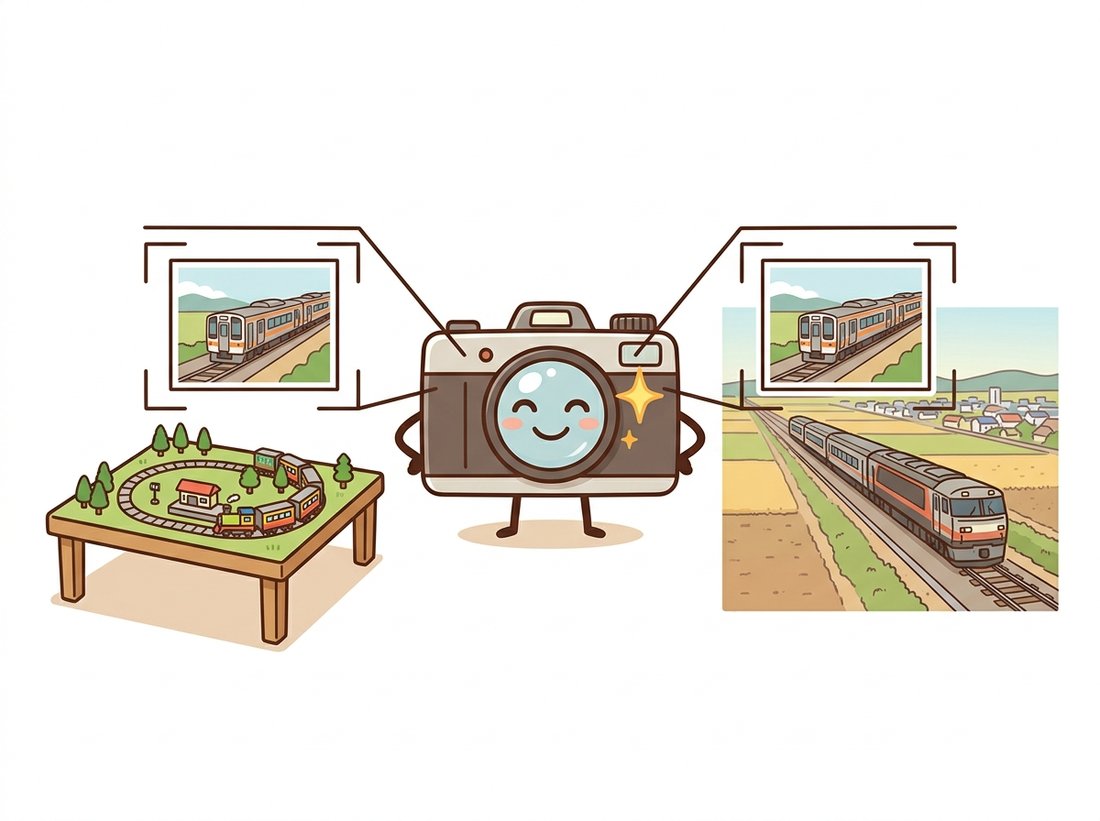
This is exactly the trick behind every miniature special effect ever filmed. A model train set photographed at the right angle is indistinguishable from a real railway, because the camera, like a monocular depth network, has no way to know the scale. Film crews exploit the ambiguity on purpose; depth networks suffer from it by accident. The difference between Hollywood and a confused neural net is that Hollywood knew the scale all along and simply declined to tell you. The illustration below makes the trap literal: one lens, two scenes, identical pixels.

2. The Cues a Network Learns Beginner

What does the network actually key on? The same monocular cues that let a person with one eye closed still reach for a coffee cup. Figure 27.1.1 names the four that dominate. Perspective: parallel lines converge with distance, so the angle of convergence encodes depth. Relative size: a familiar object (a car, a person, a door) that appears small is far away. Texture gradient: a regular texture like grass or brick compresses as it recedes. Occlusion: if object A hides part of object B, then A is nearer. None of these is geometrically exact, but together, over millions of training images, they form a powerful prior. The network is not doing geometry; it is doing learned pattern completion constrained by how real 3D scenes project.

3. The Architecture: An Encoder-Decoder for Dense Regression Intermediate

Structurally, monocular depth estimation is a dense per-pixel regression problem, and that makes it a close cousin of the semantic segmentation you built in Chapter 24. The architecture is the same encoder-decoder shape: a convolutional or transformer encoder compresses the image into a low-resolution, high-channel feature map that captures global context (essential, because depth cues like perspective are global), and a decoder upsamples back to full resolution, fusing skip connections from the encoder so fine boundaries survive. The only differences from segmentation are the head, one continuous output channel instead of per-class logits, and the loss, the scale-invariant regression loss of subsection 1 instead of cross-entropy.

The code below sketches a compact encoder-decoder depth network on a ResNet backbone of the kind you met in Chapter 20. It is deliberately small enough to read; production models are deeper and often transformer-based, but the skeleton is identical.

# Monocular depth as dense regression: a pretrained ResNet-18 encoder
# compresses the image, an upsampling decoder restores resolution, and
# encoder skip connections feed fine detail back to keep depth edges sharp.
import torch
import torch.nn as nn
import torchvision

class DepthNet(nn.Module):
    """Encoder-decoder for monocular depth: ResNet encoder, conv decoder with skips."""
    def __init__(self):
        super().__init__()
        backbone = torchvision.models.resnet18(weights="IMAGENET1K_V1")
        # Encoder stages, kept separately so we can grab skip features.
        self.stem = nn.Sequential(backbone.conv1, backbone.bn1, backbone.relu)  # 1/2
        self.pool = backbone.maxpool                                            # 1/4
        self.enc1, self.enc2 = backbone.layer1, backbone.layer2                 # 1/4, 1/8
        self.enc3, self.enc4 = backbone.layer3, backbone.layer4                 # 1/16, 1/32

        def up(cin, cout):  # upsample-then-conv decoder block
            return nn.Sequential(
                nn.Upsample(scale_factor=2, mode="bilinear", align_corners=False),
                nn.Conv2d(cin, cout, 3, padding=1), nn.ReLU(inplace=True))
        self.dec4, self.dec3 = up(512, 256), up(256 + 256, 128)
        self.dec2, self.dec1 = up(128 + 128, 64), up(64 + 64, 32)
        self.head = nn.Sequential(up(32, 16), nn.Conv2d(16, 1, 1))  # 1 depth channel

    def forward(self, x):
        s0 = self.stem(x); s1 = self.enc1(self.pool(s0))
        s2 = self.enc2(s1); s3 = self.enc3(s2); s4 = self.enc4(s3)
        d = self.dec4(s4)
        d = self.dec3(torch.cat([d, s3], 1))   # fuse encoder skip for sharp edges
        d = self.dec2(torch.cat([d, s2], 1))
        d = self.dec1(torch.cat([d, s1], 1))
        return torch.sigmoid(self.head(d))      # in (0,1); rescale to a depth range

net = DepthNet()
print("output:", net(torch.randn(1, 3, 256, 256)).shape)  # output: torch.Size([1, 1, 256, 256])

The scale-invariant loss from subsection 1 is just as compact. The implementation below operates on log-depth and matches the formula exactly; it is the supervision signal you pair with the network above when ground-truth depth (from a laser scanner or RGB-D sensor) is available.

# Scale-invariant log-depth loss (Eigen et al. 2014): penalize the variance
# of the log-error so a uniform scale offset costs nothing, which is what lets
# one network train across scenes whose absolute depths differ wildly.
def scale_invariant_loss(pred, target, mask, lam=0.85):
    """pred, target: depth maps (>0). mask: valid-pixel boolean. Eigen et al. 2014."""
    d = torch.log(pred[mask]) - torch.log(target[mask])   # per-pixel log error
    n = d.numel()
    return (d ** 2).mean() - lam * (d.sum() ** 2) / (n ** 2)

# With lam close to 1 the loss is fully scale-invariant; lam<1 keeps a little
# absolute-scale pressure, which helps when some weak metric supervision exists.

4. Training Without Ground Truth: Self-Supervision from Video Intermediate

Ground-truth depth is expensive: it needs a LiDAR rig or an RGB-D camera, and those produce sparse, noisy, indoor-biased data. The breakthrough that scaled monocular depth was learning without any depth labels, using only ordinary video or stereo pairs. The idea, from Godard and colleagues, exploits a geometric identity you already know: if you knew the depth of every pixel in frame $t$ and the camera's motion to frame $t+1$, you could warp frame $t$ to predict what frame $t+1$ should look like. The network is trained to make that prediction match the real frame $t+1$. Depth is never supervised directly; it is supervised through the photometric reconstruction error it produces.

Concretely, the network predicts depth $\hat{z}$ for the source frame and a small pose network predicts the relative camera motion $T$ between frames. Each source pixel $p_s$ is back-projected to 3D using $\hat{z}$ and the intrinsics $K$ (from Chapter 12), transformed by $T$, and reprojected into the target frame:

Sampling the target image at those reprojected coordinates gives a reconstruction of the source, and the photometric loss (a blend of pixel difference and structural similarity) drives both networks. The depth that minimizes the reconstruction error is, by the geometry, the correct relative depth. This is the same warping you would use in stereo, turned into a self-supervised objective, and it inherits the depth-scale ambiguity of subsection 1: monocular self-supervision recovers depth only up to scale, while stereo self-supervision (with a known baseline) recovers it metrically.

import kornia
# depth_warp reprojects src into the frame of dst using predicted depth + pose.
# K: (B,3,3) intrinsics; T_src_to_dst: (B,4,4); depth_src: (B,1,H,W)
warped_src = kornia.geometry.depth.warp_frame_depth(
    image_src=dst_img, depth_dst=depth_src,
    src_trans_dst=T_src_to_dst, camera_matrix=K)
photometric = (warped_src - src_img).abs().mean()  # the self-supervision signal

5. The 2024 Foundation Models for Depth Advanced

For years, monocular depth was a per-dataset affair: a model trained on indoor scenes failed outdoors, and vice versa. The shift that changed this, beginning with MiDaS in 2020 and reaching maturity in 2024, was scale and a scale-and-shift-invariant loss that let a single model train on a mixture of dozens of datasets at once. (The scale-invariant loss of subsection 1 removes a global multiplier; the scale-and-shift-invariant version also removes a global additive offset, which matters because datasets disagree not only on units but on what zero depth means, so both degrees of freedom must be factored out before comparing.) The result is zero-shot relative depth: a model that produces a sensible, sharp relative depth map on essentially any image it is shown, including domains it never saw in training. The widely used default, Depth Anything V2 (2024, arXiv:2406.09414), was trained on roughly 595,000 high-quality synthetic labeled images plus 62 million real unlabeled images through a teacher-student loop on a DINOv2 self-supervised backbone, exactly the foundation-model recipe of Chapter 25 applied to geometry. Its late-2025 successor, Depth Anything 3 (Lin et al., 2025, arXiv:2511.10647), keeps the same plain-transformer philosophy but unifies depth, camera pose, and multi-view geometry behind a single depth-ray prediction target. On its own benchmark it reports roughly a 35 percent gain in camera-pose accuracy and a 24 percent gain in geometric accuracy over the prior feed-forward state of the art (VGGT), while still improving on Depth Anything V2 for monocular depth.

Running one is now a few lines. The Hugging Face transformers pipeline below loads Depth Anything V2 and produces a relative depth map for any image, the off-the-shelf tool that the real-estate team of subsection 2 wished they had.

# Zero-shot monocular depth with a 2024 foundation model: the Hugging Face
# pipeline downloads the weights, normalizes the input, and returns a relative
# depth map for any image, with no training or per-scene tuning.
from transformers import pipeline
from PIL import Image

# Loads a 2024 foundation depth model; "Small" runs on a CPU, "Large" needs a GPU.
depth = pipeline(task="depth-estimation",
                 model="depth-anything/Depth-Anything-V2-Small-hf")

image = Image.open("street.jpg")
result = depth(image)
result["depth"].save("street_depth.png")   # a relative-depth visualization (PIL Image)
# result["predicted_depth"] is the raw tensor; larger = nearer in this model's convention.
print(result["predicted_depth"].shape)      # e.g. torch.Size([1, 518, 518])

With a depth map in hand, by whatever route, the natural next question is where to put it. A depth map is still a 2D array; to reason about the scene in 3D, to rotate it, measure it, or feed it to a 3D network, we must lift it into an explicit three-dimensional representation. That is the subject of Section 27.2.