Learning on Point Clouds: PointNet & Successors

"They handed me a bag of three-dimensional confetti and asked what it was. No grid, no order, no edges. So I looked at every piece at once, kept only the loudest opinion about each feature, and declared it a chair. I was right, which still surprises me."

A Network That Learned to Think in Sets

Section 27.2 left us with a point cloud and a problem: the convolution that powers every network in Part III needs a regular grid of neighbors, and a point cloud has none. Voxelizing the cloud (subsection 2 of the previous section) restores the grid but pays the cubic memory curse and quantizes away fine detail. The question PointNet answered, in 2017, was whether a network could consume the raw, unordered points directly. The answer reshaped 3D deep learning, and the core trick is a beautiful piece of architectural reasoning about symmetry.

1. The Permutation Problem Beginner

Let a point cloud be a set $\{x_1, x_2, \ldots, x_N\}$ of $N$ points in 3D. A network that classifies the cloud computes some function $f(\{x_1, \ldots, x_N\})$. Because the set is unordered, $f$ must satisfy permutation invariance: shuffling the points must not change the output. A standard MLP fed the points as a flattened vector $[x_1; x_2; \ldots; x_N]$ violates this immediately, the first weight column only ever sees $x_1$, so reordering the points changes the answer. A 1D convolution along the point index fails for the same reason: it assumes the index carries meaning, and it does not.

The theorem behind PointNet is that any continuous permutation-invariant function can be approximated arbitrarily well in the form

where $h$ is a per-point transformation (applied identically to each point), MAX is an element-wise maximum over all the point features (a symmetric function, immune to order), and $\gamma$ is a final transformation of the pooled result. The MAX is doing all the work: because the maximum of a set is the same regardless of how the set is listed, the whole expression is permutation-invariant by construction. PointNet simply makes $h$ and $\gamma$ learnable multilayer perceptrons (MLPs).

Fun Note: A Committee That Only Listens to the Loudest Voice

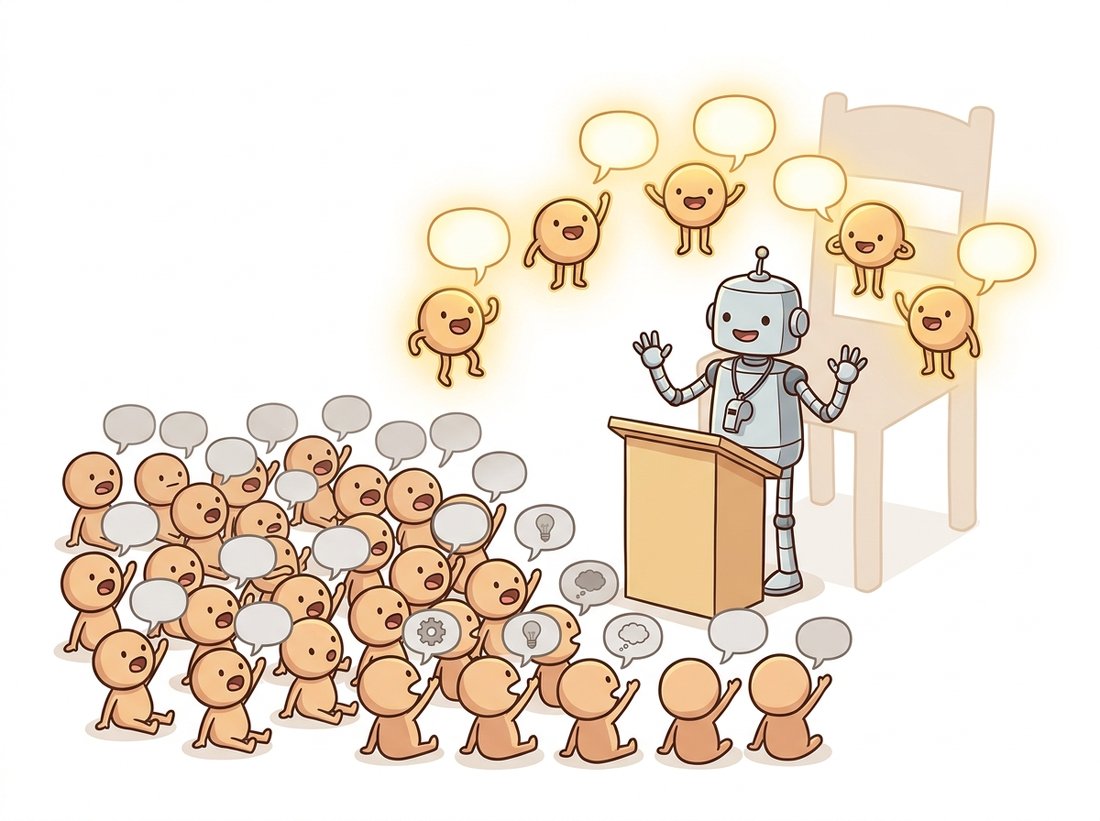
Max-pooling runs the world's most ruthless meeting. Thousands of points each shout their opinion on every feature, and for each feature the network keeps exactly one voice, the loudest, and discards the rest. The shape ends up summarized by a tiny clique of "critical points" that happened to win their channels. Delete eighty percent of the silent majority and the chair is still a chair. Democracy this is not, but it is gloriously order-independent. The illustration below stages exactly that meeting.

2. Building PointNet From Scratch Intermediate

The architecture follows the formula directly, as Figure 27.3.1 shows. Each point (an $x, y, z$ triple, plus optional features) passes through a shared MLP, implemented as a stack of $1 \times 1$ convolutions so the same weights apply to every point. After lifting each point to a high-dimensional feature, a single max-pool over the point axis produces one global feature vector for the whole cloud. For classification, that vector feeds a small MLP to class scores; for segmentation, the global feature is concatenated back onto every per-point feature so each point can be labeled using both its own identity and the global context.

The implementation below is the classification branch, complete enough to run. The crucial line is the torch.max over the point dimension, which is the symmetric aggregation of subsection 1. Read the per-point MLP as the function $h$ and the post-pool layers as $\gamma$.

# PointNet classification: a shared per-point MLP (1x1 convs) lifts each point
# to a feature vector, then a single max-pool over the point axis collapses them
# into one permutation-invariant global descriptor before the class head.
import torch
import torch.nn as nn

class PointNetCls(nn.Module):
    """PointNet classification head. Input: (B, 3, N) point clouds. Output: class logits."""
    def __init__(self, num_classes=10):
        super().__init__()
        # Shared per-point MLP as 1x1 convs: same weights applied to every point.
        self.feat = nn.Sequential(
            nn.Conv1d(3, 64, 1),   nn.BatchNorm1d(64),   nn.ReLU(),
            nn.Conv1d(64, 128, 1), nn.BatchNorm1d(128),  nn.ReLU(),
            nn.Conv1d(128, 1024, 1), nn.BatchNorm1d(1024), nn.ReLU())
        self.head = nn.Sequential(
            nn.Linear(1024, 512), nn.ReLU(), nn.Dropout(0.3),
            nn.Linear(512, num_classes))

    def forward(self, x):                  # x: (B, 3, N)
        f = self.feat(x)                   # (B, 1024, N) per-point features
        g = torch.max(f, dim=2)[0]         # (B, 1024) symmetric max-pool over points
        return self.head(g)                # (B, num_classes)

model = PointNetCls(num_classes=10)
cloud = torch.randn(4, 3, 2048)            # batch of 4 clouds, 2048 points each
print("logits:", model(cloud).shape)       # logits: torch.Size([4, 10])

# Permutation invariance check: shuffle the points, the output is unchanged.
perm = torch.randperm(2048)
same = torch.allclose(model(cloud), model(cloud[:, :, perm]), atol=1e-5)
print("invariant to point order:", same)   # invariant to point order: True

The full PointNet adds small T-Net sub-networks that predict an affine transform to align the input cloud and its features into a canonical pose, improving robustness to rotation. We omit them here for clarity; they are a refinement, not the central idea, and modern successors often drop them in favor of better local modeling.

3. Bringing Back Locality: PointNet++, DGCNN, and Point Transformers Advanced

PointNet's elegance is also its weakness. Because it pools globally in one shot, it sees each point and the whole cloud, but nothing in between: it has no notion of local neighborhoods, the very thing that made CNNs powerful through their hierarchy of receptive fields (Chapter 19). Fine geometric detail, a sharp edge, a small protrusion, is lost in the global max. The successors all answer the same question: how do you give a point-cloud network a sense of locality without a grid?

PointNet++ applies PointNet recursively. It samples a set of centroid points, gathers each one's local neighborhood (the points within a radius), runs a small PointNet on each neighborhood to summarize it, and repeats on the summarized points. This builds exactly the coarse-to-fine hierarchy of a CNN, but on sets: local features at the bottom, global structure at the top. DGCNN takes a graph view: at each layer it builds a k-nearest-neighbor graph (recomputed in feature space, hence "dynamic") and applies an edge convolution that processes each point together with its neighbors' differences, capturing relationships rather than isolated points. Point transformers (2021 onward) replace the pooling with self-attention restricted to local neighborhoods, importing the attention mechanism of Chapter 22 into 3D and currently topping most point-cloud benchmarks.

from pytorch3d.ops import sample_farthest_points, knn_points, knn_gather
# The "set abstraction" core of PointNet++ as three fused GPU operators:
# sample well-spread centroids, find each centroid's k nearest neighbors,
# and gather those neighbor coordinates into local groups for a mini-PointNet.
# points: (B, N, 3). Sample 512 well-spread centroids, then grab each one's 32 neighbors.
centroids, idx = sample_farthest_points(points, K=512)        # coverage-maximizing sample
knn = knn_points(centroids, points, K=32)                     # 32 nearest neighbors each
neighbors = knn_gather(points, knn.idx)                       # (B, 512, 32, 3) local groups
# These three calls are the "set abstraction" core of PointNet++.

We have now learned to classify and segment explicit geometry. But every method so far stores the scene as concrete points, voxels, or triangles. The most influential idea of the last five years takes a radically different route: store the entire scene inside the weights of a small neural network and recover any view by querying it. That is neural radiance fields, the subject of Section 27.4.