"They told me I could be any detector I wanted. Then they handed me a config file with four hundred lines and said the architecture was on line two hundred and twelve, inherited from a base I would have to go and read."
A Two-Stage Detector Assembled Entirely From YAML
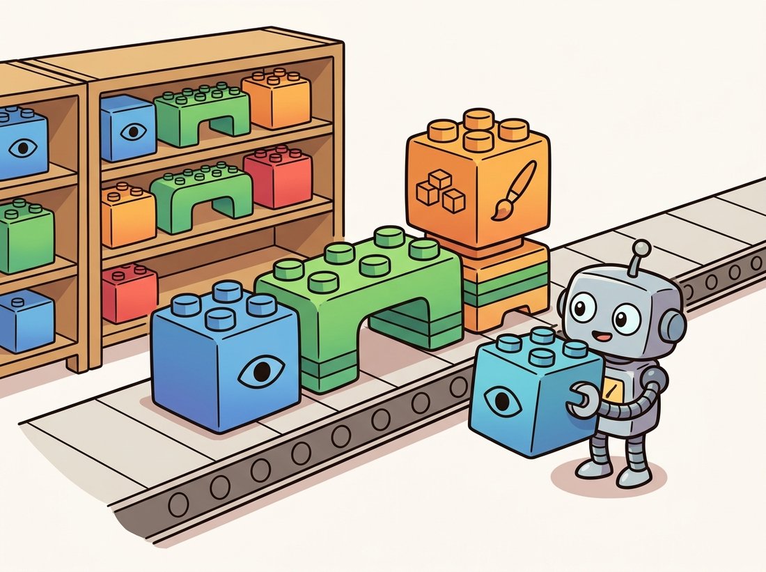
When an Ultralytics one-liner cannot express the detector you need, you move to a framework that treats a model as a composition of swappable parts described by a config file, and the two that dominate research are Detectron2 and MMDetection. Both decompose a detector into backbone, neck, and head, register every component by name, and let a text config select and wire them. The price of that flexibility is a learning curve: you trade three lines of YOLO for a config system you must learn to read. The payoff is reproducibility and control: a published result is a config you can run, and a new architecture is a few lines of config away. The illustration below shows the snap-together view of a detector that both frameworks adopt.
The moment you need a detector Ultralytics does not ship, a Swin backbone under a Cascade R-CNN head, a custom anchor scheme, a published architecture from last month's paper, the one-line API runs out of room and you are stuck. Section 29.1 ended exactly at that boundary of convenience. This section is about what you reach for instead. Detectron2 (from Meta) and MMDetection (from OpenMMLab) are the two heavyweight frameworks the research community uses to build, train, and benchmark detectors and segmenters. They share a design philosophy, decompose a model into registered, swappable modules driven by a config, and differ mostly in style and breadth. We read both config systems, compare their zoos, and end with a guide to choosing between them and the lighter tools of the previous section.
1. Why a Framework, Not a Script Intermediate
Recall the anatomy of a detector from Chapter 23: a backbone extracts features, a neck (typically a Feature Pyramid Network, or FPN) fuses them across scales, and one or more heads predict boxes and classes. A segmenter from Chapter 24 adds a mask head. The insight both frameworks exploit is that these parts are interchangeable. You can pair any backbone with any neck and any head, and most detection research is precisely such recombination. A framework that makes the parts named, registered, and config-selectable turns "try Swin instead of ResNet" from a code rewrite into a one-line config edit. Figure 29.2.1 shows the decomposition that both frameworks encode.
Count what the decomposition buys you. Suppose a framework registers just 20 backbones, 5 necks, and 10 heads, a modest fraction of what MMDetection actually ships. Because any backbone can pair with any neck and any head, that is $20 \times 5 \times 10 = 1000$ distinct detectors, each a named, runnable model, and you wrote zero of them. Add one new backbone and you have not added one model; you have added 50. This multiplicative blow-up is why a config that names three slots can express a zoo of hundreds, and why "swap ResNet for Swin" is a one-line edit rather than a fork of the codebase. The registry turns architecture research from writing models into selecting from a product space.
2. Detectron2: The Registry and the Config
Detectron2 is Meta's rewrite of the original Detectron, built on PyTorch. Its core abstraction is the registry: a lookup table that maps a string name to the Python class that builds a component, so that naming "ResNet" in a text file is enough for the framework to find and construct the right module without any import or code edit. Think of the registry as a restaurant menu: you write "ResNet" on the order slip the way a diner writes a dish name, and the kitchen (the framework) already knows which recipe (Python class) to cook, so you never touch the recipe yourself and swapping your order to "Swin" is just writing a different name, not rewriting the kitchen. The analogy stops at the door of a brand-new dish: a component nobody has registered is a dish not on the menu, which is why adding one still means writing the class and decorating it so the registry learns its name. Every backbone, head, and loss is registered under such a name, and a CfgNode config (a nested key-value tree) selects them. The library ships a model zoo of Faster R-CNN, Mask R-CNN, RetinaNet, and panoptic models, each defined by a config you can load, run, or edit. The fastest entry is the zoo plus a DefaultPredictor, which loads a config and weights and runs inference.
# Run Detectron2 inference straight from a model-zoo config: load a complete
# Mask R-CNN definition, edit one threshold on the config tree, then let a
# DefaultPredictor instantiate the model and return instance masks and classes.
from detectron2 import model_zoo
from detectron2.config import get_cfg
from detectron2.engine import DefaultPredictor
import cv2

# Start from a zoo config: Mask R-CNN with an R-50 FPN backbone, COCO-trained.
cfg = get_cfg()
zoo = "COCO-InstanceSegmentation/mask_rcnn_R_50_FPN_3x.yaml"
cfg.merge_from_file(model_zoo.get_config_file(zoo))
cfg.MODEL.WEIGHTS = model_zoo.get_checkpoint_url(zoo)   # download trained weights
cfg.MODEL.ROI_HEADS.SCORE_THRESH_TEST = 0.5             # confidence threshold

predictor = DefaultPredictor(cfg)
image = cv2.imread("street.jpg")                        # BGR, as OpenCV loads it
outputs = predictor(image)
instances = outputs["instances"]
print(instances.pred_classes)   # tensor of class indices
print(instances.pred_masks.shape)   # [N, H, W] boolean instance masks
merge_from_file loads a complete model definition; the config object is then edited in place (here, the test-time confidence threshold) before a DefaultPredictor instantiates the model and runs it. Note the BGR input convention inherited from OpenCV, the same channel-order trap from Chapter 8.
Customization happens by editing the config tree. To swap the backbone, you change cfg.MODEL.BACKBONE.NAME and the matching cfg.MODEL.RESNETS block; to train on your own data, you register a dataset (in COCO format, the standard from Chapter 23) and point cfg.DATASETS.TRAIN at it. The registry pattern means adding a brand-new head is also possible: you write the module, decorate it with @ROI_HEADS_REGISTRY.register(), and name it in the config. This is the control that the Ultralytics one-liner cannot give you.
The reason research frameworks are config-driven is reproducibility. A published detection result is not just a number; it is a specific backbone, neck, head, learning-rate schedule, augmentation policy, and random seed. When all of that lives in one text file, the result becomes runnable: anyone can merge_from_file the config, download the matching weights, and reproduce the paper. A result expressed as a custom training script with hard-coded hyperparameters scattered across functions is far harder to trust or rerun. The config file is the unit of reproducibility, which is also why it is long.
3. MMDetection: Inheritance-Based Configs Advanced
MMDetection, part of the OpenMMLab family, shares Detectron2's registry-and-config philosophy but pushes the config system further: configs inherit from base configs through a _base_ list, so a new model is often a short file that imports a base and overrides a few keys. Its model zoo is the broadest published anywhere, hundreds of detectors and segmenters spanning two-stage, single-stage, anchor-free, and transformer-based (DETR, Deformable DETR, DINO) designs, which makes it the reference for comparing architectures on equal footing.
# A custom MMDetection config: inherit a full Mask R-CNN, override a few fields.
# Saved as configs/my_mask_rcnn.py
_base_ = [
    "../_base_/models/mask-rcnn_r50_fpn.py",       # the model architecture
    "../_base_/datasets/coco_instance.py",          # dataset + pipeline
    "../_base_/schedules/schedule_1x.py",           # optimizer + LR schedule
    "../_base_/default_runtime.py",                 # logging, checkpoints
]

# Override: swap the ResNet-50 backbone for a Swin-Tiny transformer backbone.
model = dict(
    backbone=dict(
        _delete_=True,                              # drop the inherited backbone
        type="SwinTransformer",
        embed_dims=96, depths=[2, 2, 6, 2], num_heads=[3, 6, 12, 24],
    ),
    neck=dict(in_channels=[96, 192, 384, 768]),     # match Swin's channel widths
)

# Reduce the number of classes for a 3-class custom dataset.
model.update(roi_head=dict(
    bbox_head=dict(num_classes=3), mask_head=dict(num_classes=3)))
_base_ inheritance and the _delete_ flag are MMDetection's signature: a working custom model is often twenty lines because everything unmentioned is inherited from the base configs. The Swin numbers (embed_dims, depths, num_heads) are not values you memorize; they are the published Swin-Tiny size settings, copied from that architecture's reference config, and the matching neck channel widths simply restate the four feature-map widths Swin-Tiny produces.
The inheritance model is powerful and, at first, confusing: to understand a config you must trace its _base_ chain, and the architecture you are editing may be defined two files away. The payoff is that swapping a CNN backbone for the Swin transformer of Chapter 22, or swapping a two-stage head for a DETR-style set-prediction head, really is a short override. MMDetection's breadth makes it the natural home when you want to benchmark a new idea against many baselines under one training harness.
Reading an MMDetection config is the closest computer vision comes to debugging a deeply inherited object-oriented class hierarchy, except the superclass lives in a different file and the constructor argument you are hunting for was overridden three _base_ levels up. Practitioners joke that the real model zoo is not the checkpoints but the configs, and that the way you tell a senior MMDetection user from a junior one is whether they reach for a checkpoint or for a recursive config printer first. The mental model that survives: a config is a method resolution order for architectures.
| Dimension | Detectron2 | MMDetection |
|---|---|---|
| Origin | Meta AI Research | OpenMMLab |
| Config style | Flat CfgNode tree, edited in place | Python files with _base_ inheritance |
| Zoo breadth | Focused, well-curated (R-CNN family, RetinaNet, panoptic) | Very broad (hundreds, incl. DETR/DINO and transformer detectors) |
| Ecosystem | Standalone, plus DensePose and projects | OpenMMLab suite (MMSegmentation, MMPose, MMCV share conventions) |
| Learning curve | Moderate; one config file to read | Steeper; trace the inheritance chain |
| Best for | Production-leaning R-CNN work, clean API | Broad architecture benchmarking, transformer detectors |
Table 29.2.1 captures the practical split. Detectron2's flatter configs and curated zoo make it the gentler framework for someone who wants a strong Mask R-CNN with a clean Python API; MMDetection's inheritance and enormous zoo make it the reference for research that compares many architectures or needs a transformer-based detector that Detectron2 does not ship.
Building a Mask R-CNN by hand means implementing the region proposal network, the region-of-interest (ROI) align operation, the box and mask heads, the anchor matching, the multi-task loss, and the COCO-format data loading, comfortably over a thousand lines, plus weeks of debugging to match a published mAP. In either framework the same model is a config that inherits a base and overrides the class count, perhaps twenty lines, and it arrives with COCO-pretrained weights and a tested training loop. The framework handles the proposal logic, the ROI ops, the loss balancing, the augmentation pipeline, and the evaluation against COCO metrics. From-scratch construction is how Chapter 23 taught the anatomy; a real custom detector is a config edit.
4. The mAP Connection
Both frameworks report results in mean Average Precision, the detection metric defined in Chapter 23, and they compute it identically because both adopt the official COCO evaluation. Recall that mAP averages precision over recall levels and over Intersection-over-Union thresholds; COCO's primary metric averages over IoU from $0.5$ to $0.95$ in steps of $0.05$, written $\text{mAP}_{0.5:0.95}$.
The strictness of that range is easy to underestimate, so trace one box through it. Suppose a predicted box overlaps the true box at IoU $0.6$. It counts as a correct detection at the $0.5$ threshold, but it misses at every threshold from $0.7$ upward, so it earns credit in only 3 of the 10 averaged thresholds. That visually-decent box therefore scores barely above 0.3 on this metric. That is why a number like $40$ percent $\text{mAP}_{0.5:0.95}$ is a strong result, not a failing grade: most of the "missing" 60 points are boxes that look right but are not pixel-tight.
When you compare a config you trained against a published number, you are comparing on this exact protocol, which is why framework-reported numbers are directly comparable across papers in a way that ad-hoc evaluation scripts never are. This standardization is itself a reason to use a framework rather than roll your own evaluation.
It is tempting to read a leaderboard, pick the detector with the highest $\text{mAP}_{0.5:0.95}$ on COCO, and assume it is the best choice for your project. In fact COCO mAP measures one thing: average box-and-mask quality across COCO's eighty everyday-object classes, averaged over many IoU thresholds, on COCO's image distribution. It says little about how the model behaves on your classes, your image domain (medical scans, aerial tiles, factory parts), or your single operating point (one confidence threshold, one IoU you actually care about). A model two mAP points lower on the leaderboard can win decisively on your data, and a model that tops COCO can collapse on a domain it never saw. Treat mAP as a comparison protocol for ranking architectures under equal conditions, not as a verdict on fitness for your task; the only number that settles that is mAP measured on your own labeled validation set, which is exactly what the data tooling of Section 29.3 exists to produce honestly.
5. Choosing Among the Three Tiers
You now have three tiers for detection and segmentation: the Ultralytics one-liner from Section 29.1, and the two frameworks here. The decision ladder is short. If a YOLO architecture meets your accuracy and latency needs and you want results today, use Ultralytics. If you need a non-YOLO architecture, a custom component, or a faithful reproduction of a published config, use a framework. Between the frameworks, choose Detectron2 for clean R-CNN-family work and MMDetection for broad benchmarking or transformer detectors. The cost rises with the tier, more concepts, more config to read, but so does control, and the right tier is the lowest one that can express what you need.
A drone-inspection company shipped a fast YOLO detector for spotting corrosion on bridges and it worked well until a client demanded instance masks, not just boxes, to measure the affected area in square centimeters. The team tried to bolt a mask head onto their Ultralytics pipeline and fought the abstraction for a week. A senior engineer moved the project to Detectron2, started from the mask_rcnn_R_50_FPN_3x zoo config, registered their COCO-format corrosion dataset, set num_classes to two, and had instance masks training by the second day, with the COCO mAP evaluation telling them honestly where the model was weak (thin hairline cracks, the hardest class). The lesson was about tier selection: the one-liner was the right tool for the original boxes-only problem and the wrong tool the moment the requirement grew a mask head. Recognizing when you have outgrown a tier is a skill in itself, and moving up a tier early is cheaper than fighting the wrong abstraction.
The frameworks are tracking a shift away from the hand-designed anchor-and-NMS pipeline (the anchor boxes and non-maximum suppression duplicate-removal step from Chapter 23, which keeps the highest-scoring box and discards overlapping ones) toward set-prediction transformers and promptable models. The DINO and Co-DETR detectors (2023) that top the COCO leaderboards ship as MMDetection configs, making the strongest published detectors reproducible by config edit. On the segmentation side, Meta's SAM 2 (2024) generalized the promptable Segment Anything model to video and is distributed through the Hugging Face Hub of Section 29.1 rather than as a framework config, a sign that the very largest models increasingly live on hubs while the configurable frameworks remain the home for trainable, composable detectors. The 2024-2025 open-vocabulary detectors (Grounding DINO, YOLO-World) blur the line further by accepting text prompts, connecting the detection frameworks here to the vision-language models of Chapter 25. The durable skill is reading and editing a config; the architectures inside it keep turning over.
6. Summary
When convenience runs out, you reach for a framework that treats a detector as a composition of registered, config-selectable parts. Detectron2 offers a flat config and a curated R-CNN-family zoo with a clean API; MMDetection offers inheritance-based configs and the broadest zoo, including transformer detectors. Both decompose models into backbone, neck, and head, both evaluate on the official COCO mAP that makes results comparable, and both turn a custom detector from a thousand-line build into a twenty-line config edit. Choose the lowest tier that expresses your need. With models loaded and detectors composed, the remaining bottleneck is rarely the model; it is the data. Section 29.3 turns to the annotation, versioning, and visual-debugging tooling that decides your real accuracy ceiling.
An MMDetection config begins with _base_ = ["../_base_/models/faster-rcnn_r50_fpn.py", "../_base_/datasets/coco_detection.py", "../_base_/schedules/schedule_2x.py", "../_base_/default_runtime.py"] and then defines only model = dict(roi_head=dict(bbox_head=dict(num_classes=5))). In a short paragraph, describe what the final assembled model is: which backbone, neck, head, dataset, optimizer, and schedule it uses, and which single thing the override changes. Explain why this is harder to read than a self-contained config but easier to maintain across many experiments.
Using Detectron2, load the mask_rcnn_R_50_FPN_3x zoo config and run inference on a test image to confirm it works. Then edit the config to use a ResNet-101 backbone instead of ResNet-50 (change the backbone depth and load the matching zoo config or weights), and run inference again. Compare the detected instances and the per-image inference time. Report what changed in the config to make the swap and discuss the accuracy-versus-speed trade you observed, relating it to the architecture-scaling discussion of Chapter 20.
For each of the following three projects, decide whether to use Ultralytics, Detectron2, or MMDetection, and justify each choice in two or three sentences: (a) a hackathon demo that must detect people in a webcam feed in real time, finished tonight; (b) a research paper proposing a new neck design that must be benchmarked against ten published detectors under one harness; (c) a production pipeline that needs instance segmentation masks with a custom backbone and must reproduce a specific published mAP. Note any licensing or reproducibility considerations that influence your answers.