Hierarchical VAEs: From Ladder Networks to NVAE

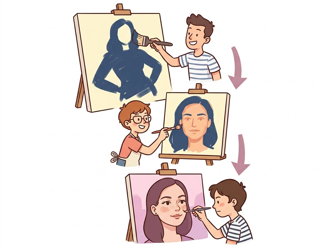
"One latent tried to remember the whole portrait at once: the pose, the freckles, the glint in the eye. It got the gist and smudged the rest. So we hired a committee, one for the silhouette, one for the cheeks, one for the eyelashes, and finally the face came back."

A Hierarchy of Latents That Learned to Delegate

In Section 31.3 and Section 31.4 the latent was a single flat vector. That design has a structural limit: every aspect of an image, from "this is a face seen in three-quarter view" down to "this eyelash curls slightly," must be packed into one code and decoded in one shot. Maximum likelihood with a Gaussian decoder then averages over the fine details it cannot pin down, which is why VAE faces come out soft. A hierarchy fixes this by giving the model multiple latent layers, top latents for global decisions and bottom latents for local detail, with each conditioned on the ones above. This section builds that idea up from the flat VAE. The illustration below pictures the hierarchy as a coarse-to-fine painting team.

1. Why One Latent Layer Is Not Enough Intermediate

Consider what a single 20-dimensional code must do for a face image. It has to specify pose, identity, lighting, expression, hairstyle, and every fine texture, all in twenty numbers, and the decoder must expand all of that simultaneously. There are two failures here. First, capacity: twenty numbers cannot carry both the global plan and the local detail, so detail is sacrificed. Second, structure: the model has no way to express that "given the pose and identity (global), the eyelashes (local) follow," a conditional structure that real images obviously have. A hierarchy of latents $z_1, z_2, \ldots, z_L$ addresses both. The generative model factorizes top-down,

so the topmost latent $z_L$ is drawn from the prior and decides global structure, each lower latent is drawn conditioned on the one above and refines the picture, and the decoder finally renders the image from the bottom latent. Coarse-to-fine generation falls out naturally: the top of the stack lays out the silhouette, the bottom fills in texture, exactly the multi-resolution decomposition of a Laplacian pyramid but with learned, stochastic levels.

2. The Ladder VAE and Bidirectional Inference Advanced

Training a deep latent stack runs into a hard problem on the inference side. A naive encoder that simply mirrors the generative model bottom-up tends to leave the upper latents undertrained: the gradient signal reaching $z_L$ is weak, and those latents collapse toward the prior (the posterior collapse of Section 31.4, now striking the top of the hierarchy first). The ladder VAE solves this with a bidirectional inference path. A bottom-up deterministic pass extracts features at every level; then a top-down stochastic pass computes each latent's posterior by combining the bottom-up features with the top-down generative prediction from the layer above. In effect the encoder and the generative model share their top-down pathway, so the posterior at each level is a precision-weighted merge (precision is the inverse of variance, so a more confident, lower-variance source gets a larger weight in the blend) of "what the data says" (bottom-up) and "what the layers above expect" (top-down). This coupling is what gives the upper latents a strong, well-conditioned signal and keeps them alive. Figure 31.5.1 contrasts the flat VAE with the ladder's two coupled passes.

The next block sketches one level of a hierarchical VAE, showing how the top-down prior for a level and the bottom-up data features are combined to form that level's posterior. The full model stacks these cells; the snippet isolates the coupling that defines the ladder.

# One level of a ladder VAE: form this level's posterior by merging the
# top-down conditional prior p(z_l | z_{l+1}) with bottom-up data features.
# Stacking L of these cells, each fed bottom-up features, is the hierarchy.
import torch
import torch.nn as nn

class LadderLevel(nn.Module):
    """One level: combine top-down prior with bottom-up evidence."""
    def __init__(self, dim):
        super().__init__()
        self.prior = nn.Linear(dim, 2 * dim)     # p(z_l | z_{l+1}): mu, logvar
        self.merge = nn.Linear(2 * dim, 2 * dim)  # combine with bottom-up features

    def forward(self, top_down, bottom_up):
        p_mu, p_logvar = self.prior(top_down).chunk(2, dim=-1)      # from above
        q_params = self.merge(torch.cat([top_down, bottom_up], -1))
        q_mu, q_logvar = q_params.chunk(2, dim=-1)                  # posterior
        std = torch.exp(0.5 * q_logvar)
        z = q_mu + std * torch.randn_like(std)    # reparameterized sample
        # KL between this level's posterior q and its conditional prior p:
        kl = 0.5 * (p_logvar - q_logvar + (q_logvar.exp() + (q_mu - p_mu) ** 2)
                    / p_logvar.exp() - 1).sum(-1)
        return z, kl
# Stacking L of these, with bottom-up features feeding each level, is the
# hierarchical VAE. The per-level KL is to the CONDITIONAL prior p(z_l|z_{l+1}),
# not to N(0, I), which is the key difference from the flat VAE.

3. NVAE and the Engineering of Depth Advanced

The ladder fixed the inference structure, but pushing the stack to the dozens of latent groups needed for high-resolution images exposed raw optimization instability: the KL terms across many levels are hard to balance, activations explode or vanish, and the model diverges. NVAE (2020) is the recipe that tamed this, and it is worth knowing the ingredients because the same problems recur in any very deep generative model. Three design choices carry the weight:

• Residual latent cells, built from depthwise-separable convolutions and squeeze-and-excitation blocks (the efficiency primitives of Chapter 28), so signal flows cleanly through depth as in a ResNet.
• Spectral regularization plus careful normalization, bounding the Lipschitz constant of each layer (the Lipschitz constant is the largest factor by which a layer can stretch the distance between two inputs, so bounding it caps how violently the layer can amplify a change), which keeps the KL terms smooth and prevents the sharp instabilities that otherwise kill deep VAEs.
• A residual posterior parameterization that expresses each level's distribution as a small offset from its prior, which both stabilizes the KL and counters collapse.

The companion "Very Deep VAE" work (2021) made a complementary point. A clean hierarchical VAE, made deep enough, outperforms the autoregressive PixelCNN-class models on likelihood. (PixelCNN generates an image one pixel at a time, each pixel conditioned on those already produced above and to the left.) The lesson was that depth in the latent stack, not architectural exotica, was the missing ingredient.

4. Where Hierarchical VAEs Sit Now Intermediate

Hierarchical VAEs occupy an important conceptual position even though pure diffusion now leads on raw image fidelity. Their deep top-down generative path, coarse latents conditioning fine ones, is structurally the same coarse-to-fine refinement that diffusion performs over time steps, and several works draw the equivalence explicitly: a diffusion model can be read as a particular very deep hierarchical VAE whose latents are the noisy intermediates and whose per-step decoders share weights. Understanding the hierarchical VAE therefore demystifies a large part of Chapter 33 in advance. In practice, the hierarchy idea persists in the multi-resolution latent designs used inside modern image and video autoencoders, and the depth-stabilization tricks NVAE introduced reappear wherever a generative stack must be trained deep. The next block shows how to read off the coarse-to-fine behavior by sampling the top latents and resampling the bottom ones.

# Read off the hierarchy's coarse-to-fine behavior: hold the top (global)
# latent fixed and resample only the lower latents, so the outputs share
# global structure but vary in fine texture, one control per scale.
import torch

# Demonstrate coarse-to-fine control in a trained hierarchical VAE.
model.eval()
with torch.no_grad():
    z_top = torch.randn(1, top_dim)            # fix the GLOBAL latent
    variations = []
    for _ in range(8):
        # Resample only the lower (fine-detail) latents, keep z_top fixed.
        img = model.generate(z_top=z_top, resample_lower=True)
        variations.append(img)
    # The 8 images share global structure (same pose/identity, set by z_top)
    # but differ in fine texture (set by the resampled lower latents).
    # This is the hierarchy made visible: each scale is a separate control.