Inside Stable Diffusion: VAE, U-Net, DiT & Conditioning

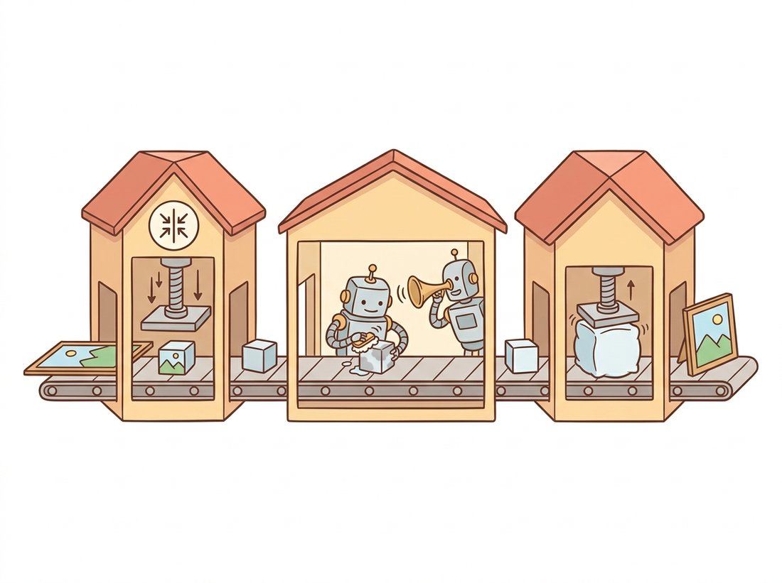
"I am three machines pretending to be one product. One shrinks the world to a thumbnail nobody is meant to see, one paints inside that thumbnail while a sentence whispers what to draw, and one enlarges the result and takes the bow. The poster only has room for 'Stable Diffusion'."

A Latent Diffusion Stack Maintaining a United Front

In Section 34.1 we produced the conditioning sequence: a tensor of per-token text embeddings. This section is about the machine that consumes it. We assemble the three components of latent diffusion that Chapter 33 introduced separately, show how cross-attention threads the text through the denoiser, and run the assembled system so the abstract pipeline becomes a concrete sequence of tensor shapes.

1. Three Stations and the Tensor Between Them Beginner

The architecture is a pipeline, and Figure 34.2.1 is the map. Text goes into the frozen encoder of Section 34.1 and comes out as a conditioning sequence. A random latent is denoised by the U-Net over many steps, with the conditioning injected at every step through cross-attention. The finished latent is decoded to pixels by the VAE decoder. The pixel-space image never touches the denoiser; all the expensive iteration happens in the small latent, which is the entire reason latent diffusion fits on a consumer GPU. The cartoon below gives the same map a friendlier face: three machines in a row.

2. The Autoencoder: Compress, Then Decode Intermediate

The first and last stations are the same network: the variational autoencoder you built in Chapter 31, here used as a fixed perceptual compressor. Stable Diffusion's VAE maps a $512 \times 512 \times 3$ image to a $64 \times 64 \times 4$ latent, an eightfold spatial downsampling per side and a $48\times$ reduction in element count. The latent is not a semantic code; it is a near-lossless perceptual compression, trained with a combination of reconstruction loss, a small KL penalty toward a standard normal, and an adversarial term (the GAN discriminator of Chapter 32) that keeps decoded textures sharp. The diffusion process then runs entirely in this $64 \times 64 \times 4$ space.

The compression ratio is the lever. A diffusion step on a $64 \times 64$ grid costs a fraction of a step on a $512 \times 512$ grid, so latent diffusion buys roughly an order-of-magnitude speedup over pixel diffusion at the same image resolution. There is a fixed scaling factor (0.18215 for the SD 1.x VAE) applied when moving between the VAE's natural output and the unit-variance scale the denoiser expects. The denoiser was trained on latents normalized to roughly unit variance, so it only behaves correctly when its input arrives at that same scale; forgetting the factor feeds it latents at the wrong magnitude and produces washed-out or over-saturated images, a classic first-day bug.

import torch
from diffusers import AutoencoderKL
from diffusers.utils import load_image
import torchvision.transforms.functional as TF

# Encode an image to the compact latent the denoiser works in, then
# decode it back, to make the eightfold-per-side compression concrete.
# The scaling_factor moves between VAE space and the denoiser's variance.
vae = AutoencoderKL.from_pretrained(
    "stable-diffusion-v1-5/stable-diffusion-v1-5", subfolder="vae").eval()

img = load_image("https://huggingface.co/datasets/huggingface/"
                 "documentation-images/resolve/main/diffusers/cat.png")
x = TF.to_tensor(img.resize((512, 512))).unsqueeze(0) * 2 - 1   # to [-1, 1]

with torch.no_grad():
    latent = vae.encode(x).latent_dist.sample() * vae.config.scaling_factor
    recon = vae.decode(latent / vae.config.scaling_factor).sample

print("pixel input:", tuple(x.shape))        # (1, 3, 512, 512)
print("latent code:", tuple(latent.shape))   # (1, 4, 64, 64)
print("compression (elements):",
      x.numel() // latent.numel(), "x")

The print confirms the shapes promised in subsection 1: a $(1, 4, 64, 64)$ latent is what the denoiser actually sees. Everything in the next two subsections happens in this compact space.

3. The Denoiser and Cross-Attention Advanced

The denoiser is the only learned, time-dependent part of the loop and the place the text exerts its influence. In classic Stable Diffusion it is a U-Net: the convolutional encoder-decoder with skip connections whose convolution lineage runs back to Chapter 3. The U-Net takes the noisy latent $z_t$, a timestep embedding $t$, and the text conditioning, and predicts the noise $\epsilon_\theta(z_t, t, c)$ to remove. What makes it text-aware are the cross-attention blocks inserted at several resolutions.

Cross-attention is the self-attention of Chapter 22 with the keys and values coming from a different source than the queries. Here the queries come from the image latent (each spatial position asks a question) and the keys and values come from the text conditioning sequence (each word offers an answer):

$$ \text{CrossAttn}(Q_{\text{image}}, K_{\text{text}}, V_{\text{text}}) = \text{softmax}\!\left(\frac{Q_{\text{image}} K_{\text{text}}^\top}{\sqrt{d}}\right) V_{\text{text}}. $$

Each spatial location in the latent computes an attention distribution over the prompt's tokens and pulls in a weighted blend of their value vectors. This is precisely how the word "fox" can influence the latent positions that will become the fox and leave the background tokens to influence the snow. The attention maps are interpretable: visualizing the attention weight from the "fox" token to every spatial position produces a soft segmentation of where the model is placing the fox, which is the hook that later editing methods in Chapter 35 grab onto.

import torch, torch.nn.functional as F
from torch import nn

# Cross-attention is where text enters the denoiser: image-latent
# positions form the queries, the text tokens form keys and values,
# so every spatial cell pulls in a weighted blend of word vectors.
class CrossAttention(nn.Module):
    """Image-latent queries attend to text keys/values (single head, for clarity)."""
    def __init__(self, img_dim, txt_dim, d):
        super().__init__()
        self.to_q = nn.Linear(img_dim, d, bias=False)   # from image latent
        self.to_k = nn.Linear(txt_dim, d, bias=False)   # from text conditioning
        self.to_v = nn.Linear(txt_dim, d, bias=False)
        self.scale = d ** -0.5

    def forward(self, x, context):
        # x: (B, HW, img_dim) spatial tokens;  context: (B, L, txt_dim) text tokens
        q, k, v = self.to_q(x), self.to_k(context), self.to_v(context)
        attn = (q @ k.transpose(-2, -1)) * self.scale     # (B, HW, L)
        attn = attn.softmax(dim=-1)                       # each pixel over words
        return attn @ v, attn                             # also return the maps

ca = CrossAttention(img_dim=320, txt_dim=768, d=320)
latent_tokens = torch.randn(1, 64 * 64, 320)              # flattened 64x64 latent
text_ctx = torch.randn(1, 77, 768)                        # CLIP conditioning
out, maps = ca(latent_tokens, text_ctx)
print("output:", tuple(out.shape), "attention maps:", tuple(maps.shape))

3.1 From U-Net to Diffusion Transformer

The U-Net is not the only choice of denoiser. The diffusion transformer (DiT) of Chapter 33 replaces the convolutional backbone with a pure transformer: the latent is split into patches, flattened into a token sequence, and processed by transformer blocks. DiT scales more predictably than the U-Net (its quality improves smoothly with compute, the same scaling behavior that drove the language-model era) and it folds text conditioning in naturally because it already speaks tokens. SD3 and FLUX use a DiT variant, MMDiT, in which image tokens and text tokens flow through the same attention blocks as a joint sequence rather than the image querying the text from a separate stream. The denoiser's job, predict the noise given the noisy latent, timestep, and text, is identical; only the internal wiring changes.

4. One Full Generation, Traced Intermediate

We now assemble the three stations into a single manual generation, calling the components directly rather than the convenience pipeline, so every tensor that crosses a station boundary is visible. This is the code to read when a pipeline misbehaves and you need to inspect an intermediate.

import torch
from diffusers import (StableDiffusionPipeline, UNet2DConditionModel,
                       AutoencoderKL, DDIMScheduler)
from transformers import CLIPTokenizer, CLIPTextModel

# Run the three stations by hand instead of through a pipeline, so every
# tensor that crosses a station boundary (encoder, U-Net loop, VAE) is
# visible. This is the version to read when a generation misbehaves.
device, dtype = "cuda", torch.float16
repo = "stable-diffusion-v1-5/stable-diffusion-v1-5"
tok = CLIPTokenizer.from_pretrained(repo, subfolder="tokenizer")
enc = CLIPTextModel.from_pretrained(repo, subfolder="text_encoder").to(device, dtype)
unet = UNet2DConditionModel.from_pretrained(repo, subfolder="unet").to(device, dtype)
vae = AutoencoderKL.from_pretrained(repo, subfolder="vae").to(device, dtype)
sched = DDIMScheduler.from_pretrained(repo, subfolder="scheduler")

prompt = "a red fox sitting in fresh snow, sharp focus, soft daylight"
guidance = 7.5

# 1. Encode prompt and an empty string for classifier-free guidance.
def embed(text):
    ids = tok(text, padding="max_length", max_length=77,
              truncation=True, return_tensors="pt").input_ids.to(device)
    return enc(ids)[0]
cond, uncond = embed(prompt), embed("")
ctx = torch.cat([uncond, cond])                       # (2, 77, 768)

# 2. Start from pure latent noise and set the denoising schedule.
sched.set_timesteps(30, device=device)
z = torch.randn(1, 4, 64, 64, device=device, dtype=dtype) * sched.init_noise_sigma

# 3. The denoising loop.
for t in sched.timesteps:
    inp = sched.scale_model_input(torch.cat([z, z]), t)        # duplicate for CFG
    with torch.no_grad():
        eps_u, eps_c = unet(inp, t, encoder_hidden_states=ctx).sample.chunk(2)
    eps = eps_u + guidance * (eps_c - eps_u)                   # classifier-free guidance
    z = sched.step(eps, t, z).prev_sample

# 4. Decode the final latent to pixels.
with torch.no_grad():
    img = vae.decode(z / vae.config.scaling_factor).sample
print("final latent:", tuple(z.shape), "-> image:", tuple(img.shape))

That loop is the whole system. Every named product in Section 34.3 is a variation on it: a different encoder feeding ctx, a different denoiser computing eps, a different scheduler stepping z. The classifier-free guidance blend in step 3 is the prompt-strength control that Section 34.5 dissects.

# The same forty lines of manual generation, packed into one call:
# the pipeline runs the encoder, the CFG-duplicated denoising loop,
# the scaling factor, and the VAE decode internally.
from diffusers import StableDiffusionPipeline
import torch

pipe = StableDiffusionPipeline.from_pretrained(
    "stable-diffusion-v1-5/stable-diffusion-v1-5", torch_dtype=torch.float16).to("cuda")
image = pipe("a red fox sitting in fresh snow, sharp focus",
             num_inference_steps=30, guidance_scale=7.5).images[0]