Spatial Control: ControlNet & Conditioning Adapters

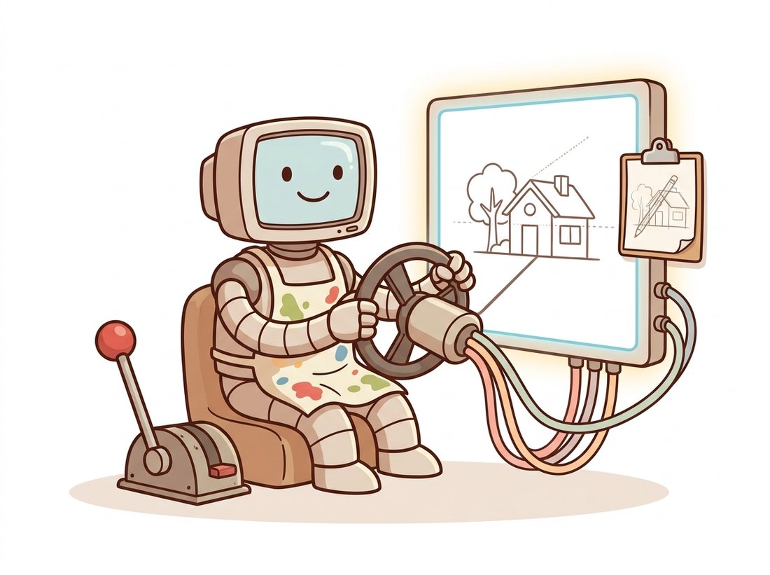
"Tell me what to draw and I will improvise wildly. Show me where to draw it and I will suddenly become very professional."

A Diffusion U-Net With a Newfound Respect for Structure

In Chapter 34 the only handle on a generation was the text prompt, and a prompt is a poor instrument for geometry. You can write "a cathedral" but not "this exact silhouette"; you can write "a person waving" but not "this precise pose." Spatial control closes that gap. Given a structural map derived from a reference (or drawn by hand), a controlled model produces an image whose layout matches the map and whose content matches the prompt. This section builds the mechanism: first the ControlNet architecture and its zero-convolution trick, then the conditioning signals (edges, depth, pose) that come straight from earlier chapters, then the lighter adapter alternatives, and finally the conditioning-scale dial that decides how strictly the model obeys. The opening illustration below captures the shift this chapter makes.

1. The Problem: Prompts Cannot Specify Geometry Beginner

Recall from Section 34.2 how text reaches the image: the prompt is encoded into a sequence of token embeddings, and cross-attention layers in the U-Net let every spatial location query those embeddings. This is a powerful but fundamentally global and semantic channel. The word "left" in a prompt nudges a soft statistical prior; it does not place a pixel. If you need the horizon at row 200, a hand in the lower-right quadrant, or the same composition as a reference photo, no amount of prompt wording reliably delivers it, because the conditioning signal carries meaning, not coordinates.

The fix is to add a conditioning signal that is spatial: a map with the same height and width as the latent grid, where each location carries a structural hint. An edge map says "there is a boundary here." A depth map says "this region is near, that one is far." A pose skeleton says "the elbow is at this coordinate." The model is then trained so that the generated image respects the map. Figure 35.1.1 contrasts the two conditioning channels.

2. ControlNet: A Trainable Copy of the Encoder Intermediate

The naive way to add spatial conditioning would be to fine-tune the whole U-Net on (control map, image) pairs. This is expensive and risky: with limited control data you can damage the rich generative prior that took millions of images to learn, a catastrophic-forgetting failure of exactly the kind Chapter 21 warned about during transfer learning. ControlNet sidesteps the risk with a clean architectural move. It freezes the original U-Net entirely and creates a trainable copy of just the encoder half (the downsampling blocks). The control map is fed into this copy. The copy's outputs are added back into the frozen U-Net's decoder at the corresponding resolutions.

The crucial detail is how the copy connects to the frozen network. Each connection passes through a zero convolution: a $1 \times 1$ convolution whose weights and bias are initialized to zero. Because a zero-initialized layer outputs zero regardless of input, at the very first training step the control branch adds nothing, and the controlled model produces exactly what the original model would. Let $\mathcal{F}$ be a frozen block with parameters $\Theta$, let $\mathcal{F}_c$ be its trainable copy with parameters $\Theta_c$, and let $\mathcal{Z}(\cdot;\,\cdot)$ be a zero convolution. The controlled output of a block on feature $x$ with control input $c$ is

At initialization both zero convolutions output zero, so $y_c = \mathcal{F}(x;\Theta)$ exactly: the network is unchanged. Gradients still flow into the zero convolutions (their input is nonzero), so they begin to learn immediately, but they grow from a safe starting point rather than injecting random noise into a delicate pretrained model. This is why ControlNet trains stably on datasets of only tens of thousands of pairs and rarely degrades the base model's quality. Figure 35.1.2 shows the wiring.

3. Conditioning Signals: Edges, Depth, Pose Intermediate

A ControlNet is trained for one type of control map, so there is a ControlNet for Canny edges, another for depth, another for OpenPose skeletons, and so on. The beautiful part is that the maps themselves come directly from techniques earlier in this book. The Canny edge map is exactly the Canny detector of Chapter 9; the depth map is the output of a monocular depth network from Chapter 27; the pose skeleton is a keypoint detector. The code below uses diffusers to run a Canny-conditioned ControlNet end to end: detect edges, then generate an image that follows them.

# Canny-conditioned ControlNet, end to end: detect edges on a reference,
# then generate an image whose layout follows those edges while the prompt
# decides material and lighting. The edge map is the geometric channel.
import cv2
import numpy as np
import torch
from PIL import Image
from diffusers import StableDiffusionControlNetPipeline, ControlNetModel

# 1. Build the Canny control map from a reference image (Chapter 9 detector).
ref = cv2.imread("reference.jpg")
edges = cv2.Canny(ref, 100, 200)                 # low/high hysteresis thresholds
edges = np.stack([edges] * 3, axis=-1)           # ControlNet expects 3 channels
control = Image.fromarray(edges)

# 2. Load a Canny ControlNet alongside a base Stable Diffusion model.
controlnet = ControlNetModel.from_pretrained(
    "lllyasviel/sd-controlnet-canny", torch_dtype=torch.float16)
pipe = StableDiffusionControlNetPipeline.from_pretrained(
    "stable-diffusion-v1-5/stable-diffusion-v1-5", controlnet=controlnet,
    torch_dtype=torch.float16).to("cuda")

# 3. Generate: the prompt sets content, the edge map sets layout.
image = pipe(
    "a sandstone temple at golden hour, photorealistic",
    image=control,
    num_inference_steps=30,
    controlnet_conditioning_scale=1.0,            # full obedience to edges
).images[0]
image.save("controlled.png")

Swapping the control type is a two-line change: load sd-controlnet-depth with a depth map, or sd-controlnet-openpose with a pose skeleton. The depth ControlNet is the practitioner's favorite for relighting and style transfer because depth preserves three-dimensional structure while letting surfaces change freely; the pose ControlNet is the standard tool for putting a character in a chosen stance. Because the maps are the very outputs you learned to compute in Parts II and III, the controllable generator is the point where the classical and deep pipelines of this book feed into the generative one.

4. Lighter Alternatives: T2I-Adapter and IP-Adapter Advanced

ControlNet clones half the U-Net, which roughly doubles the parameters that must be loaded and run. Two adapter families trade a little control fidelity for a much smaller footprint. T2I-Adapter uses a small standalone convolutional network (a few million parameters, not a U-Net copy) that extracts features from the control map and adds them into the encoder once, rather than at every block. It is cheaper to train and to run and is strong enough for edge, depth, and sketch control, though slightly less precise than ControlNet on hard structural constraints.

IP-Adapter ("image prompt adapter") solves a different problem: conditioning on an image rather than a structural map. It encodes a reference image with CLIP (the CLIP encoder of Chapter 25) and adds a decoupled cross-attention path, a second set of attention layers that attend to the image embedding in parallel with the text cross-attention. This lets you say "generate in the style of this picture" or "keep this face" by supplying an example image alongside the text. The decoupling is what makes it compose cleanly: the text path and the image path each have their own attention, so the model can follow a prompt and a reference image at once. The snippet shows IP-Adapter style conditioning.

# IP-Adapter conditioning: condition on a reference IMAGE rather than a
# structural map. CLIP encodes the reference and a decoupled cross-attention
# path lets the model follow both the text prompt and the picture at once.
from diffusers import StableDiffusionPipeline
from diffusers.utils import load_image
import torch

pipe = StableDiffusionPipeline.from_pretrained(
    "stable-diffusion-v1-5/stable-diffusion-v1-5", torch_dtype=torch.float16).to("cuda")

# Attach an IP-Adapter: a decoupled image cross-attention path.
pipe.load_ip_adapter("h94/IP-Adapter", subfolder="models",
                     weight_name="ip-adapter_sd15.bin")
pipe.set_ip_adapter_scale(0.6)                   # how strongly the image prompt acts

style_ref = load_image("style_reference.png")    # the image to imitate
image = pipe(
    prompt="a fox sitting in a forest clearing",
    ip_adapter_image=style_ref,                  # image conditioning, not a control map
    num_inference_steps=30,
).images[0]

5. The Conditioning-Scale Dial Intermediate

Every control method exposes a single most important hyperparameter at inference time: how strongly the control signal acts. In ControlNet it is controlnet_conditioning_scale, a multiplier $\lambda$ applied to the control branch's contribution before it is added into the frozen U-Net. The illustration below makes the tradeoff concrete. Writing the controlled block output with the scale made explicit,

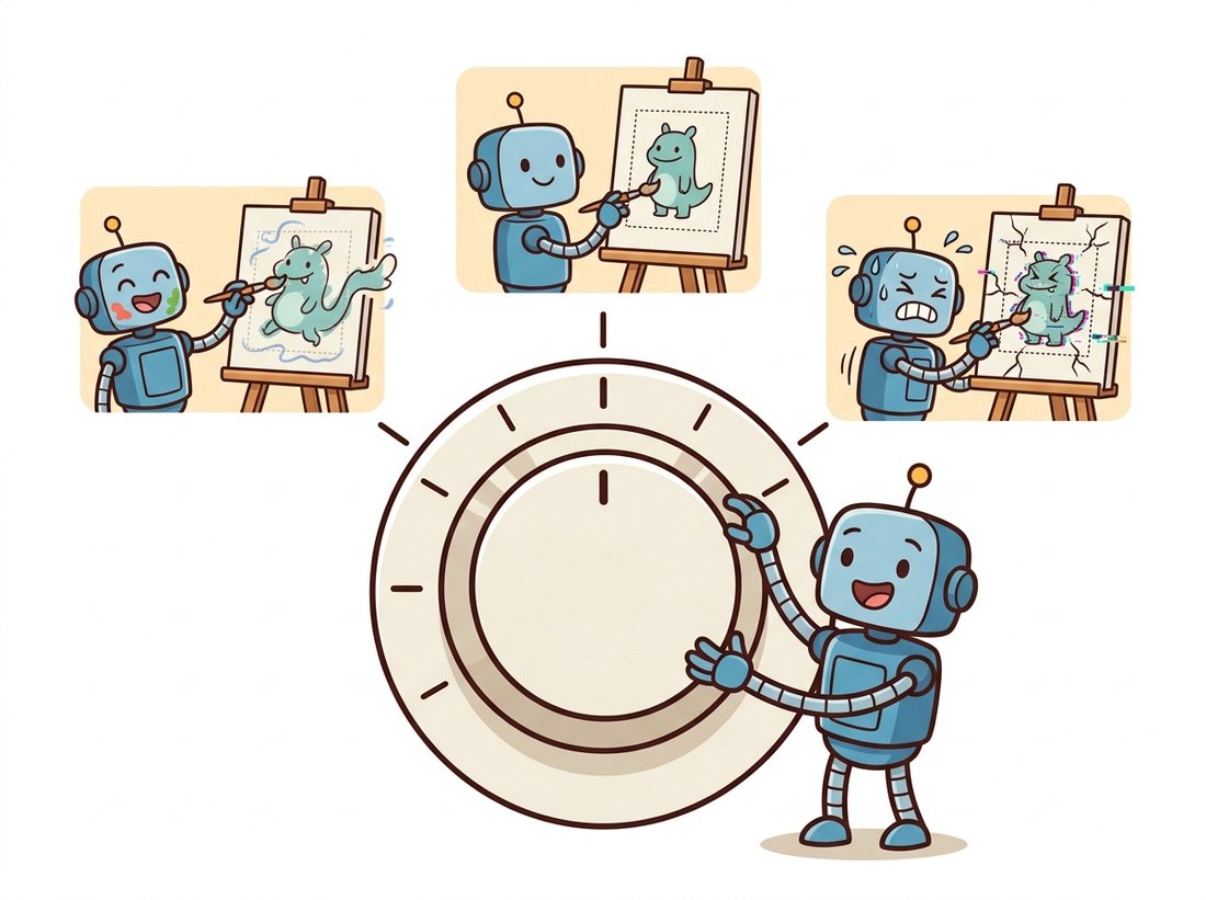
At $\lambda = 0$ the control branch is silent and you get an ordinary text-to-image generation. At $\lambda = 1$ the model follows the structure as trained. Pushing beyond $1$ forces ever-stricter adherence to the map, at the cost of artifacts where the prompt and the structure disagree (the model is being asked to satisfy a geometry that its content prior resists). Below $1$ the structure becomes a suggestion the model may bend. The right value depends on the task: a precise architectural render wants $\lambda$ near $1.0$, while loose compositional guidance often looks best near $0.5$. There is also a guidance start and end control that applies the conditioning only during a window of the sampling steps, since the early steps fix coarse layout and the late steps add detail. The one-line rule of thumb to remember is obedience, not quality: $\lambda$ trades how strictly the map is followed against how freely the prompt invents, and the best setting is the smallest $\lambda$ that pins the structure you care about.