Video Diffusion: Architectures & Temporal Consistency

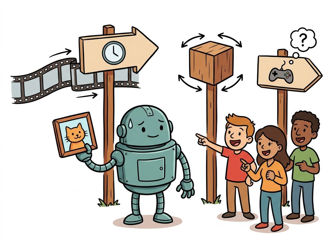
"Drawing one cat is easy. Drawing the same cat sixty times in a row, without it sprouting a third ear in frame 31, turns out to be the entire job."

A U-Net That Learned to Count Frames

In Chapter 33 you trained a model to take a noisy image and predict the noise, then ran that prediction in a loop to sculpt clean pixels out of Gaussian static. Chapter 34 conditioned that loop on a text prompt through cross-attention. If you simply run such an image model independently on each frame of a video, you get a catastrophe that the field calls flicker: each frame is individually plausible, but the texture of a wall, the pattern on a shirt, the exact shade of the sky, all jitter chaotically from frame to frame because nothing forces consecutive frames to agree. The previous section's tools, optical flow and temporal modeling from Chapter 26, told you how to read motion; this section is about how to generate it consistently. The illustration below frames the whole leap: drawing one good frame is easy, and the real job is making it agree across time, across viewpoints, and with the actions you take.

1. From Image Denoiser to Video Denoiser Intermediate

A video is a tensor of shape $(B, F, C, H, W)$: batch, frames, channels, height, width. An image diffusion U-Net or diffusion transformer (DiT) operates on $(B, C, H, W)$. The cheapest possible video model treats the frame axis as part of the batch, denoising every frame independently. This is the flicker baseline, and its failure is instructive: the denoiser has no pathway through which the pixel at $(t, x, y)$ can be influenced by the pixel at $(t-1, x, y)$. The fix is to add exactly such a pathway. Two designs dominate, and modern models use both.

Temporal attention reshapes the tensor so that, for each fixed spatial location, the $F$ frames form a sequence, then applies self-attention along that sequence. A pixel in frame 30 can now look at the same pixel in frames 1 through 60 and copy or blend their values. Temporal (3D) convolution instead slides a small kernel along the time axis, mixing a frame with its immediate neighbors, cheaper than attention and excellent for local motion smoothness. The influential factorized design from Ho et al.'s Video Diffusion Models paper keeps the expensive spatial layers exactly as in the image model and interleaves cheap temporal layers between them, so an image checkpoint can be inflated into a video model by inserting and lightly training the temporal blocks.

Figure 36.1.1 shows the factorized block. The code below implements a minimal version of the temporal-attention insert, the single most important component, as a module you can drop after any spatial attention layer.

# Temporal-attention insert: couples the same spatial location across all
# frames so an image denoiser becomes frame-consistent. Dropped in after each
# spatial-attention block; the residual keeps it near-identity at init.
import torch
import torch.nn as nn
from einops import rearrange

class TemporalAttention(nn.Module):
    """Self-attention along the time axis, applied per spatial location.
    Drop this in after a spatial-attention block to make frames consistent."""
    def __init__(self, dim, n_heads=8):
        super().__init__()
        self.attn = nn.MultiheadAttention(dim, n_heads, batch_first=True)
        self.norm = nn.LayerNorm(dim)

    def forward(self, x, num_frames):
        # x arrives as (B*F, C, H, W); regroup so time becomes the sequence axis
        bf, c, h, w = x.shape
        x = rearrange(x, "(b f) c h w -> (b h w) f c", f=num_frames)  # tokens = frames
        residual = x
        x = self.norm(x)
        x, _ = self.attn(x, x, x)          # each pixel attends across all F frames
        x = residual + x                    # residual keeps the spatial signal intact
        x = rearrange(x, "(b h w) f c -> (b f) c h w", h=h, w=w)
        return x

block = TemporalAttention(dim=320, n_heads=8)
video = torch.randn(2 * 16, 320, 32, 32)   # batch 2, 16 frames, 320-ch latents
out = block(video, num_frames=16)
print(out.shape)   # torch.Size([32, 320, 32, 32]); shape preserved, frames now coupled

The shape gymnastics in the rearrange calls are the whole trick. Spatial attention treats $(H \cdot W)$ as the sequence and $F$ as batch; temporal attention swaps them, treating $F$ as the sequence and $(H \cdot W)$ as batch. The residual connection is essential: it guarantees that adding an untrained temporal layer to a pretrained image model is initially a near-identity operation, so the image model's quality is preserved while the temporal layer learns motion.

2. The Video VAE: Compressing Time Intermediate

Generating a 5-second clip at 24 frames per second and 512-by-512 resolution means 120 frames of about 786,000 color values each ($512 \times 512 \times 3 = 786{,}432$): nearly 100 million numbers. Running diffusion directly in pixel space at that scale is infeasible, which is exactly the problem latent diffusion solved for images in Chapter 33 by working inside a VAE's compressed latent space. Video pushes the idea further: a video VAE compresses not only each frame spatially (the usual 8-by-8 factor) but also temporally, encoding several consecutive frames into one latent frame using 3D convolutions in the encoder and decoder.

A typical modern video VAE applies a temporal compression of 4 on top of an 8-by-8 spatial compression. A 120-frame clip becomes about 30 latent frames; the $786{,}432$ color values per frame become $64 \times 64 \times 4 = 16{,}384$ latent values. The total compression factor is $8 \times 8 \times 4 = 256$, and the diffusion transformer then operates entirely on these compact spacetime latents. This is the same move that the latent-space view of Chapter 31 made for single images, now extended along the clock.

One design detail makes the temporal compression usable in practice: the 3D convolutions are causal in time. Each temporal kernel looks only at the current and past frames, never future ones, and the very first frame is padded against itself so it can be encoded alone. This buys two things. It lets the model stream and extend a clip without re-encoding the whole timeline, and, crucially, it makes a single image a valid one-frame clip, so the same VAE encodes both stills and video. That joint image-and-video capability is exactly what lets systems like Stable Video Diffusion and SD3-era video models pretrain on abundant images and fine-tune on scarcer video through one shared latent space.

# Load a pretrained video VAE instead of building one: the same from_pretrained
# interface as the image VAE. This particular VAE uses a temporal-aware decoder,
# so reconstruction stays smooth across frames before diffusion does any work.
from diffusers import AutoencoderKLTemporalDecoder
# The temporal-decoder VAE shipped with Stable Video Diffusion.
vae = AutoencoderKLTemporalDecoder.from_pretrained(
    "stabilityai/stable-video-diffusion-img2vid-xt", subfolder="vae")
latents = vae.encode(frames).latent_dist.sample()   # 4-channel spatial latents, 8x downsampled

3. Temporal Consistency: The Central Battle Advanced

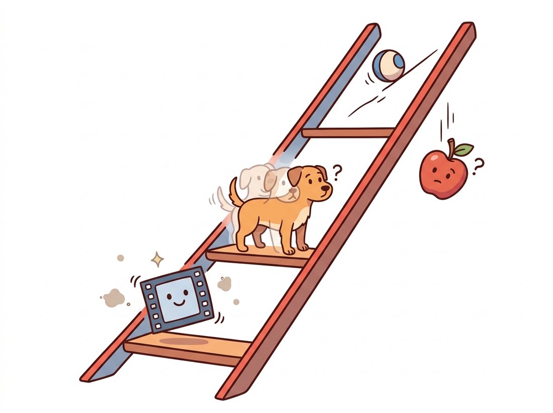
With architecture and VAE in place, the real engineering is fighting the failure modes of consistency. There are three, and they fail at different time scales. The illustration below ladders them by time scale, from a quick frame-to-frame twitch up to physics that quietly refuses to hold.

High-frequency flicker is the frame-to-frame jitter of texture and color. It is fought by the temporal attention and 3D convolution of Section 1, which directly couple adjacent frames. Identity drift is slower: over a few seconds, a face slowly morphs, a logo on a shirt mutates, a dog's breed changes. This is a long-range problem; local temporal layers cannot fix it because frame 1 and frame 120 never directly attend to each other unless the attention window spans the whole clip. Motion incoherence is the third: objects that teleport, limbs that pass through bodies, water that flows uphill. This is the deepest failure, and it is really the world-modeling problem that Sections 36.5 through 36.8 confront head-on; a video model that produces coherent motion has implicitly learned some physics.

A practical and widely used diagnostic borrows directly from Chapter 26: measure consistency with optical flow. Warp each frame forward into the next frame's coordinates using the predicted flow, and measure how much the warped frame disagrees with the actual next frame. Low warping error means the content moved coherently; high error means flicker or teleportation. This warping-error metric is the workhorse quantitative check, and it formalizes the loop closed by the cross-reference map: optical flow, introduced classically in Chapter 15 and learned in Chapter 26, becomes the ruler for video generation here.

# Quantify temporal consistency by re-deriving each frame from its predecessor:
# warp frame t into frame t+1 via dense optical flow, then measure the residual.
# A low score means motion is coherent; a high score flags flicker or teleportation.
import cv2
import numpy as np

def temporal_warping_error(frames):
    """Mean per-pixel error after warping each frame into the next via optical flow.
    Low value = temporally consistent; high value = flicker or teleportation."""
    gray = [cv2.cvtColor(f, cv2.COLOR_RGB2GRAY) for f in frames]
    errors = []
    for t in range(len(frames) - 1):
        # dense Farneback flow from frame t to frame t+1
        flow = cv2.calcOpticalFlowFarneback(
            gray[t], gray[t + 1], None, 0.5, 3, 15, 3, 5, 1.2, 0)
        h, w = gray[t].shape
        # build the sampling grid that pulls frame t forward by the flow
        grid_x, grid_y = np.meshgrid(np.arange(w), np.arange(h))
        map_x = (grid_x + flow[..., 0]).astype(np.float32)
        map_y = (grid_y + flow[..., 1]).astype(np.float32)
        warped = cv2.remap(frames[t], map_x, map_y, cv2.INTER_LINEAR)
        errors.append(np.abs(warped.astype(float) - frames[t + 1]).mean())
    return float(np.mean(errors))

# A perfectly consistent clip approaches the camera/codec noise floor;
# an independently-denoised (flickering) clip scores several times higher.
print(f"warping error: {temporal_warping_error(my_clip):.2f}")

The diffusers ecosystem will not compute this for you, so the snippet above is the kind of evaluation glue you write yourself; it is also the seed of the world-model evaluation in Section 36.8, where physical-plausibility probes generalize this idea well beyond optical flow.

4. Conditioning and the Image-to-Video Special Case Intermediate

Most practical video generation is conditioned: on a text prompt (text-to-video, the subject of Section 36.2), on a starting image (image-to-video, which animates a photo), or on both. Image-to-video is the most reliable mode today and the most instructive. The conditioning image is encoded by the VAE and concatenated to the noisy latents of every frame, so the denoiser always has the ground-truth first frame to anchor against. This anchoring directly attacks identity drift: because every frame can attend back to a clean encoding of the subject, the face or logo has a fixed reference and wanders far less.

The same classifier-free guidance you met in Chapter 34 applies, with a twist: video models often expose a motion-bucket or guidance-strength control that trades off motion magnitude against stability. Crank it up and the video moves dramatically but risks incoherence; turn it down and you get a stable, nearly still clip. This is the controllability knob that Chapter 35's philosophy of steerable generation extends into the temporal domain, and it is the bridge to action-conditioned generation in the world-model sections, where the conditioning signal becomes a control input rather than a static image.

5. Putting It Together Beginner

The full video-diffusion recipe is now a short list, each item a piece you already understand from earlier chapters. Encode the clip into spacetime latents with a video VAE (the latent idea from Chapter 31). Add noise on a schedule (the forward process from Chapter 33). Denoise with a spatiotemporal transformer or U-Net whose spatial layers come straight from the image model and whose temporal layers (Section 1) couple the frames. Condition on text via cross-attention (Chapter 34) or on an image via concatenation (Section 4). Decode the denoised latents back to pixels with the video VAE. Evaluate consistency with a flow-based warping metric (Section 3). The novelty over an image model is entirely concentrated in the temporal layers and the temporal compression; the rest is diffusion you already built.

That concentration is the reassuring takeaway and the bridge forward. You do not need a new theory of generation to make video; you need a way for frames to talk to each other and a compressed clock to do it efficiently. Section 36.2 scales exactly this recipe up, replacing the U-Net with a latent transformer and the fixed clip length with arbitrary spacetime patches, to reach the Sora-class systems and the open models you can run today.