"They told me I was one model. Then they opened me up and found a scheduler, a U-Net, a VAE, a text encoder, and a tokenizer, all pretending to be a single function call. I have never felt so seen, or so disassembled."
A Text-to-Image Pipeline During Its First Code Review
Hugging Face Diffusers is the central library of generative vision because it presents the same system at two altitudes: a one-line pipeline for people who want an image, and a set of swappable components (scheduler, denoiser, VAE, text encoder) for people who want to change how the image is made. Learning to drop from the pipeline to its parts, and back, is the core fluency of the Python generation stack, and it maps one-to-one onto the diffusion theory of Chapter 33.
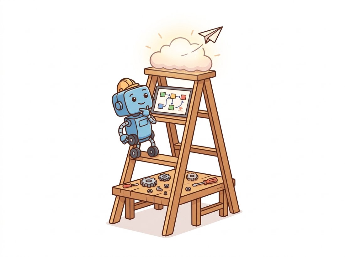
Throughout Part IV the library hiding behind the math was almost always Diffusers. Chapter 33 built a sampler loop by hand and then noted the DiffusionPipeline that does it in one call; Chapter 34 assembled a latent-diffusion system whose four parts Diffusers exposes as named attributes; Chapter 35 attached a LoRA and a ControlNet that Diffusers loads with one method each. This section is the pause that names the library, takes a pipeline apart, and shows the ecosystem around it (PEFT, Accelerate, Transformers) that turns a research checkpoint into something that runs on the GPU you actually own. The recurring theme is that a "model" here is never one object; it is a small society of objects, and control comes from knowing each one's job. The illustration below frames the whole chapter as a three-rung ladder.
1. The Pipeline Abstraction Beginner
The highest-altitude entry point is the pipeline. A DiffusionPipeline bundles every component needed to go from a text prompt to an image: the text encoder and tokenizer, the denoising network, the variational autoencoder (VAE) that decodes latents to pixels, the scheduler that defines the sampling trajectory, and the safety and post-processing glue. You name a checkpoint on the Hub, the pipeline downloads and wires all of it, and a single call produces an image. Figure 38.1.1 shows the components a pipeline assembles and the order in which a generation flows through them.
The code that drives Figure 38.1.1 is deliberately short. The pipeline takes a checkpoint identifier, a prompt, and a handful of generation parameters, and returns an image. The half-precision and device placement are the only lines that betray that a multi-gigabyte model is involved.
import torch
from diffusers import DiffusionPipeline

# Load a complete text-to-image system by Hub checkpoint id.
# torch_dtype=float16 halves memory; variant picks the fp16 weight files.
pipe = DiffusionPipeline.from_pretrained(
    "stabilityai/stable-diffusion-xl-base-1.0",
    torch_dtype=torch.float16,
    variant="fp16",
)
pipe = pipe.to("cuda")

# A single call runs the full prompt-to-image trajectory.
image = pipe(
    prompt="a cinematic photo of a lighthouse in a storm, dramatic light",
    num_inference_steps=30,        # number of scheduler steps
    guidance_scale=6.5,            # classifier-free guidance strength
    generator=torch.Generator("cuda").manual_seed(0),  # reproducible
).images[0]

image.save("lighthouse.png")
print(type(pipe).__name__)   # StableDiffusionXLPipeline
from_pretrained downloads and wires every component; the call runs the sampling loop. num_inference_steps and guidance_scale are the two knobs from Chapter 34: how many denoising steps to take, and how hard to push toward the prompt. A fixed generator seed makes the result reproducible.
The two generation knobs are exactly the ones Chapter 33 and Chapter 34 derived. num_inference_steps is the number of points at which the scheduler evaluates the reverse process; more steps trace a finer trajectory at higher cost. guidance_scale is the classifier-free guidance weight $w$, which interpolates between the unconditional and conditional score predictions as $\hat{\epsilon} = \epsilon_\varnothing + w\,(\epsilon_\text{cond} - \epsilon_\varnothing)$; larger $w$ binds the image more tightly to the prompt at the cost of diversity and, past a point, realism. Nothing about the library hides this math; it just spares you the loop.
Newcomers often treat num_inference_steps like an image-quality dial that always pays off if turned up, the same instinct that makes people believe a higher-resolution capture is always sharper. It is not. The step count is how finely the scheduler discretizes the reverse-diffusion trajectory of Chapter 33, and once the discretization is fine enough to track that fixed continuous path, extra steps add compute and change essentially nothing in the image. A good solver like DPMSolverMultistepScheduler reaches that plateau near 20 to 30 steps, and few-step distilled models reach it at 1 to 4; pushing a 30-step pipeline to 150 steps mostly buys you a longer wait. Steps choose how accurately you walk a path, not how good the destination is; the destination is fixed by the trained denoiser and the guidance setting.
Take Code Fragment 1 and change nothing but guidance_scale, holding the prompt, the seed, and num_inference_steps fixed. Generate the same prompt at roughly 1.5, 4, 7, 12, and 20, and lay the five images side by side. Watch two things move together: as you climb, the image binds harder to the prompt and color saturation and contrast rise, then past the upper end detail flattens and skin and sky go waxy and oversaturated, the same failure the field story below diagnoses. Because the seed is fixed, every difference you see is the guidance weight $w$ in $\hat{\epsilon} = \epsilon_\varnothing + w\,(\epsilon_\text{cond} - \epsilon_\varnothing)$ and nothing else. Most SDXL-class models have a sweet spot around 5 to 8; finding where your prompt starts to degrade teaches that knob faster than any paragraph, and it costs five short generations.
2. The Component Model: Taking the Pipeline Apart Intermediate
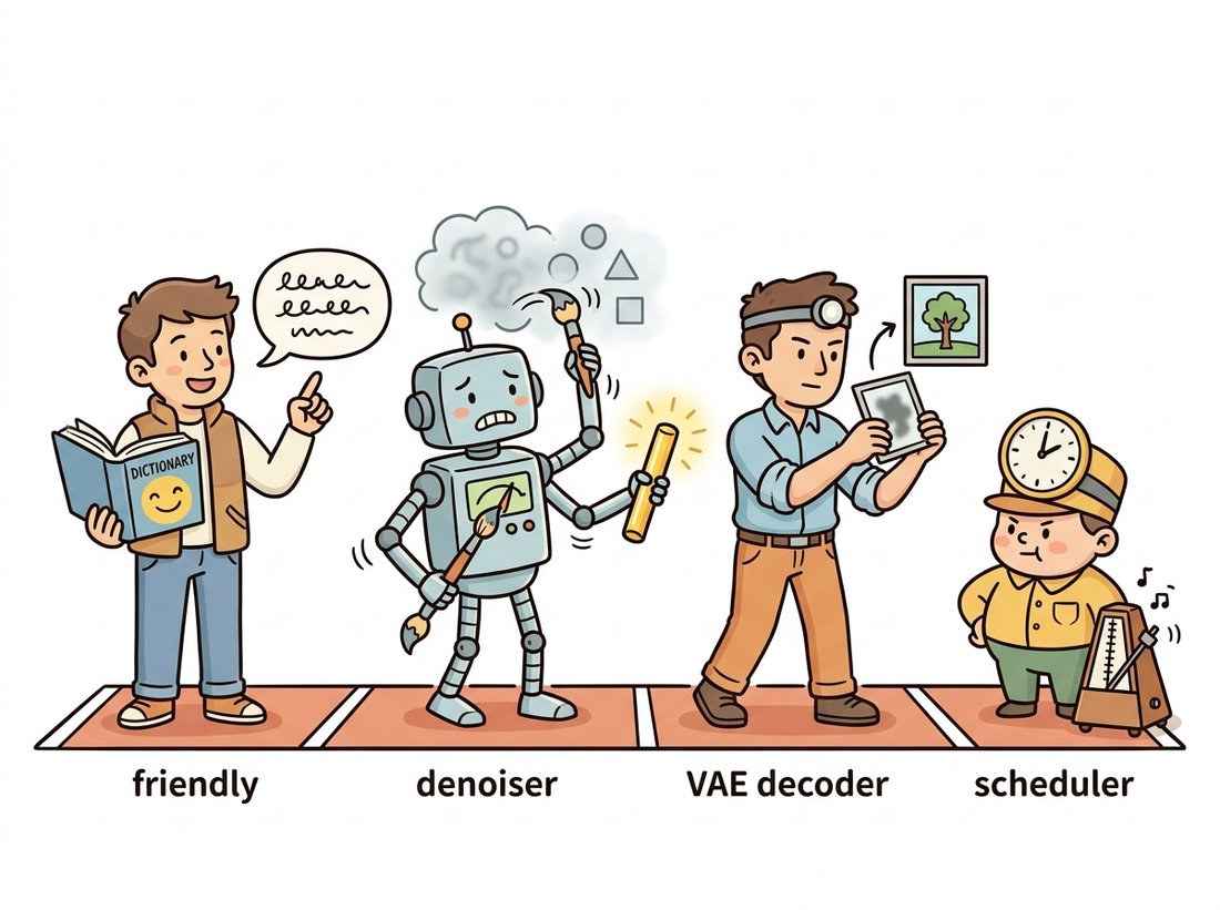
The reason Diffusers is the central library rather than one of several is the component model. A loaded pipeline is not a black box; it is a container whose parts are accessible as attributes, pipe.unet, pipe.vae, pipe.scheduler, pipe.text_encoder, and each can be inspected, reconfigured, or replaced with a compatible object. The most common and most instructive swap is the scheduler, because it changes the sampler from Chapter 33 without touching the trained weights at all. Picture the pipeline as the relay team in the illustration below, where each runner owns one leg of the work.
from diffusers import DiffusionPipeline, DPMSolverMultistepScheduler

pipe = DiffusionPipeline.from_pretrained(
    "stabilityai/stable-diffusion-xl-base-1.0", torch_dtype=torch.float16
).to("cuda")

# Inspect the components: each is a real, named object you can reach.
print(pipe.unet.config.sample_size)        # latent spatial size, e.g. 128
print(pipe.scheduler.__class__.__name__)   # EulerDiscreteScheduler (default)

# Swap the sampler. DPM-Solver++ reaches good quality in fewer steps.
# from_config reuses the noise schedule the model was trained with.
pipe.scheduler = DPMSolverMultistepScheduler.from_config(pipe.scheduler.config)

image = pipe("a watercolor fox", num_inference_steps=20).images[0]
from_config is the critical detail: it inherits the trained noise schedule (betas, prediction type) so the new sampler solves the same reverse process the model expects, rather than a mismatched one.
That from_config call carries a lesson worth stating plainly. The scheduler and the denoiser share a contract: the noise schedule the model trained against. A scheduler built from a fresh config with default betas would solve a slightly different differential equation than the one the U-Net learned to reverse, and the images would degrade for no obvious reason. This is the diffusion-era cousin of the preprocessing-mismatch bug from the deep-vision stack in Chapter 29: the model and the thing wrapped around it must agree on a shared convention, and the library gives you a method that copies that convention rather than making you retype it.
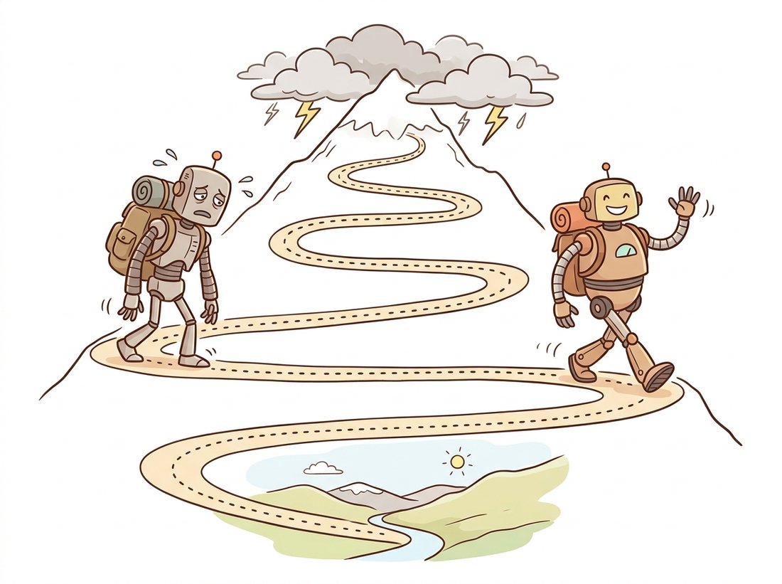
A scheduler in Diffusers contains no learned parameters. It is a numerical integrator for the reverse-diffusion ordinary or stochastic differential equation, and swapping EulerDiscreteScheduler for DPMSolverMultistepScheduler is the same kind of move as swapping a first-order ODE solver for a higher-order one. The mechanism behind "better integrator" is concrete: plain Euler uses only the denoiser prediction at the current step and assumes the trajectory is locally straight, so it accumulates error and needs many small steps to stay on the curved path; a multistep solver like DPM-Solver++ reuses the predictions it already computed at the previous one or two steps to estimate the path's curvature, which lets each step be larger while staying accurate. That is why a faster sampler can cut num_inference_steps from 50 to 20 with little visible loss: it extracts more information per denoiser call from the same trajectory, not a different model. The denoiser weights, the part that took thousands of GPU-hours to train, are completely unchanged. The illustration below makes the picture literal: two hikers, the same trail.
The same accessibility extends to the other components. You can replace the VAE with a higher-fidelity decoder, freeze the text encoder while fine-tuning the U-Net, or load a different denoiser entirely as long as it speaks the same latent shape. Modern flagship checkpoints increasingly replace the U-Net denoiser with a diffusion transformer (DiT), and Diffusers exposes those through the same attribute named transformer instead of unet; the contract, conditioning vectors in, predicted noise out, is identical.
When a generation goes wrong, run down the components in the order data flows through them and ask which one owns the symptom: "Encoder, Denoiser, VAE, Scheduler". Garbled meaning is the text encoder; wrong content is the denoiser or its guidance; mushy or banded pixels are the VAE; speed or step-count problems are the scheduler. Four boxes, four suspects. The single most common newcomer mistake is to blame the whole "model" and swap the multi-gigabyte checkpoint when the actual culprit was a one-line scheduler or guidance setting that costs nothing to change.
3. Specializing a Generator: PEFT and LoRA
A base checkpoint is general. To make it draw your product, your art style, or your character, you do not retrain it; you attach a low-rank adapter, the LoRA technique from Chapter 35. Diffusers integrates the Hugging Face PEFT library so that loading a LoRA is one method call, and you can stack several and weight them. The transfer-learning thread that began with frozen backbones in Chapter 25 reaches its generative form here: adapt a foundation model by training a few million parameters, not a few billion.
pipe = DiffusionPipeline.from_pretrained(
    "stabilityai/stable-diffusion-xl-base-1.0", torch_dtype=torch.float16
).to("cuda")

# Attach a style LoRA from a Hub repo. weight_name picks the file.
pipe.load_lora_weights(
    "ostris/super-cereal-sdxl-lora", weight_name="cereal_box_sdxl_v1.safetensors",
    adapter_name="cereal",
)

# Multiple adapters can be combined and weighted at inference time.
pipe.set_adapters(["cereal"], adapter_weights=[0.8])

image = pipe("a cereal box for an AI startup, vibrant").images[0]

# Fuse the adapter into the base weights for faster repeated inference,
# or call pipe.unload_lora_weights() to remove it entirely.
pipe.fuse_lora()
load_lora_weights injects the low-rank adapter matrices into the denoiser's attention layers; set_adapters mixes adapters at chosen strengths; fuse_lora bakes the adapter into the base weights so repeated generation pays no per-step adapter cost.The line-count contrast with from-scratch specialization is stark, and it is exactly the "right tool" point this book makes in every chapter.
To attach a LoRA by hand you would locate every attention projection in the denoiser, wrap each nn.Linear with a parallel low-rank pair $W + \frac{\alpha}{r} B A$, register the new parameters, load the adapter tensors from a checkpoint, and handle the scaling and fusing, roughly 80 to 120 lines of careful module surgery, with a real risk of wrapping the wrong layers. The Diffusers and PEFT equivalent is pipe.load_lora_weights(repo) plus pipe.set_adapters(...): two lines. The library handles layer discovery, the rank-and-alpha math, multi-adapter mixing, and the safetensors loading. Hand-rolling the wrapper is how you learn what a LoRA is; production loads it.
4. Fitting on the GPU You Own: Accelerate and Memory
Flagship checkpoints are large. A Stable Diffusion XL (SDXL) pipeline in half precision wants roughly 10 to 12 GB of GPU memory to run comfortably, and the larger transformer-based models want more. Diffusers, built on Hugging Face Accelerate, offers a graded set of memory-versus-speed trade-offs so the same pipeline runs on a 24 GB workstation card or an 8 GB laptop GPU, just at different speeds. The knobs move components between GPU and CPU, or tile the VAE decode, rather than changing the model.
| Call | What it does | Memory saved | Speed cost |
|---|---|---|---|
pipe.to("cuda") | All components resident on GPU (baseline) | None | Fastest |
enable_model_cpu_offload() | Keep one component on GPU at a time, rest on CPU | Large | Small (a few percent) |
enable_sequential_cpu_offload() | Offload at the submodule level, finest granularity | Largest | High (much slower) |
enable_vae_tiling() | Decode the VAE in tiles to avoid a large activation | Moderate (decode only) | Small |
enable_attention_slicing() | Compute attention in chunks | Moderate | Small to moderate |
The practical recipe for a memory-constrained card is to combine the cheapest knobs first. Model CPU offload plus VAE tiling typically brings an SDXL pipeline under 8 GB with only a small speed penalty, because most of the time only the denoiser is active and the VAE decode is the single largest activation.
pipe = DiffusionPipeline.from_pretrained(
    "stabilityai/stable-diffusion-xl-base-1.0", torch_dtype=torch.float16
)
# Do NOT call .to("cuda") when offloading; offload manages placement itself.
pipe.enable_model_cpu_offload()   # one component on GPU at a time
pipe.enable_vae_tiling()          # tile the final decode

image = pipe("a misty mountain valley at dawn", num_inference_steps=25).images[0]
# Runs on an 8 GB GPU; expect a few seconds slower than the all-resident path.
enable_model_cpu_offload keeps only the active component (text encoder, then denoiser, then VAE) on the GPU; enable_vae_tiling avoids the single large decode activation. The comment flags the one real gotcha: with offload enabled you must not also call .to("cuda"), because offload owns device placement.Look at what those two lines actually buy. The all-resident SDXL pipeline wants 10 to 12 GB of VRAM, which is the line between a card you can afford and a card you cannot; model CPU offload plus VAE tiling drops that under 8 GB, enough headroom to fit a laptop GPU, and the toll is the "Small" entry in Table 38.1.1, a few percent of wall-clock. You are trading roughly a third of your memory footprint for single-digit-percent slower generation. That is the lopsided exchange rate the whole Accelerate layer exists to offer: it almost never costs speed in proportion to the memory it saves, because at any instant only one component (the denoiser, then the VAE) is actually on the GPU, and the rest is sitting in cheap system RAM doing nothing.
5. The Surrounding Ecosystem
Diffusers does not stand alone. It sits in the middle of a small constellation of Hugging Face libraries that each own one job, and fluency means knowing which library answers which question. Chapter 34's text encoder is a Transformers model; the LoRA training and loading is PEFT; the multi-GPU and offload machinery is Accelerate; and the checkpoints, adapters, and datasets all live on the Hub, reached through the huggingface_hub client. Table 38.1.2 names the division of labor.
| Library | Owns | You reach for it when |
|---|---|---|
| diffusers | Pipelines, schedulers, denoisers, VAEs | You are generating, sampling, or composing a diffusion model |
| transformers | Text encoders, tokenizers, vision-language models | You need the prompt encoder or a multimodal conditioner |
| peft | LoRA and other parameter-efficient adapters | You are specializing a generator without full fine-tuning |
| accelerate | Device placement, offload, multi-GPU, mixed precision | The model does not fit, or you are training across GPUs |
| huggingface_hub | Downloading and uploading checkpoints and adapters | You are fetching weights or publishing your own |
This division is why a generative project that would have meant one monolithic research codebase in 2021 is now a handful of imports. It also explains the most common confusion for newcomers: a question about why a prompt is encoded a certain way is a Transformers question, while a question about why the image looks oversaturated at high guidance is a Diffusers question. Knowing which library owns the behavior is half of debugging it.
A small studio building a product-photography generator reported that their SDXL outputs looked "soft and washed out" compared to the demos they had seen online, and they were about to switch to a different base model. A reviewer asked to see their generation call and found two issues in five minutes, both in the component layer. First, they were running the default 50-step Euler scheduler but had copied a guidance_scale of 12 from an old Stable Diffusion 1.5 tutorial; SDXL is tuned for guidance around 5 to 8, and the high value was over-saturating and flattening detail. Second, they were never using the SDXL refiner, the optional second denoiser stage the architecture provides for sharper fine detail. Lowering guidance to 6.5 and adding the refiner pass, both one-line component changes, not a model swap, produced the crisp images they wanted. The lesson is the component model itself: when generation looks wrong, the fix is usually a scheduler, a guidance value, or a missing stage, not a different checkpoint.
6. A Decision Guide
The altitude question, pipeline or components, is settled by how much you need to change. If you want images from prompts and the defaults are fine, stay at the pipeline level; it is one call and the maintainers have chosen sensible defaults. Drop to the component level the moment you need to swap a sampler for speed, attach an adapter for style, condition on a control map, or fit the model on a smaller GPU. Reach into the surrounding libraries by job: PEFT for adapters, Accelerate for memory and multi-GPU, Transformers for the text encoder. And when even the component model is more orchestration than you want to write in Python, that is the signal to move up to the node-based workflow engines of Section 38.2, or out to the hosted APIs of Section 38.3.
The component model is what let Diffusers absorb the 2024-2026 wave of generation research without breaking the pipeline API. Distillation methods that collapse sampling to a handful of steps, latent consistency models (Luo et al., 2023, arXiv:2310.04378) and their LoRA form, and adversarial-distilled samplers such as SDXL-Turbo and the SD3-Turbo line, ship as either a special scheduler or a loadable adapter, so a user adopts one-step or four-step generation by swapping a component, not rewriting their code. In parallel, the flagship architectures moved from the U-Net to the diffusion transformer (DiT, Peebles and Xie 2023) and to flow-matching objectives, the lineage behind the Stable Diffusion 3 and 3.5 models (the latter released in October 2024) and the FLUX family of rectified-flow transformers, whose larger FLUX.2 release of late 2025 is reported by Black Forest Labs as a roughly 32-billion-parameter flow-matching transformer paired with a vision-language encoder. Diffusers exposes these through a transformer attribute and dedicated pipelines while keeping the conditioning contract identical. The durable skill is the same one this section teaches: think of a generator as swappable components, and each year's headline method tends to arrive as a new object you can slot in.
7. Summary
Diffusers presents a generative model at two altitudes: a one-line pipeline and a set of swappable components (scheduler, denoiser, VAE, text encoder) that map directly onto the diffusion theory of Chapter 33 and the latent-diffusion architecture of Chapter 34. Swap the scheduler to change the sampler without retraining; attach a LoRA through PEFT to specialize the model; reach for Accelerate's offload knobs to fit a small GPU. The surrounding libraries each own one job, and knowing which one owns a behavior is half of debugging it. When the orchestration outgrows a Python script, the next tool is a node-based workflow engine, the subject of Section 38.2. The best way to make the component model muscle memory is to drive every knob in this section once, on one pipeline, and watch each change in isolation; put it into practice in the Hands-On Lab at the end of this section, which has you build a small generation studio that decomposes a pipeline, swaps the sampler, attaches a LoRA, fits the whole thing on an 8 GB GPU, and prices the result against a hosted Call.
A colleague swaps the default scheduler for DPMSolverMultistepScheduler and reports that 20 steps now look as good as the old 50 steps, then asks whether this means the model "got better". In three or four sentences, explain why no learned parameter changed, what a scheduler actually is in terms of the reverse-diffusion equation from Chapter 33, and why from_config (rather than a fresh config) is necessary for the swap to be valid.
Load any Stable Diffusion XL pipeline. Without generating an image, print the class name and a key config value for each of pipe.text_encoder, pipe.unet, pipe.vae, and pipe.scheduler (for example the U-Net's sample_size, the VAE's scaling_factor, and the scheduler's number of training timesteps). Then generate one image, swap only the scheduler to DPMSolverMultistepScheduler.from_config(pipe.scheduler.config), regenerate with the same seed and half the steps, and compare the two images and their wall-clock times. Report what changed and what did not.
You must run an SDXL pipeline on an 8 GB GPU. Using Table 38.1.1, design a combination of memory-saving calls that you predict will fit, and justify the order in which you would add them (cheapest speed cost first). Then state, for each knob you chose, exactly what it trades and why it helps, and explain the specific reason you must not call pipe.to("cuda") when enable_model_cpu_offload() is active. If a single knob were not enough, which would you add next and why?
Build a single, self-contained studio.py that loads one text-to-image pipeline and then exercises every concept of this chapter on it: it decomposes the pipeline into its four named components, swaps the scheduler for a faster solver, attaches a LoRA to specialize the style, fits the whole thing onto an 8 GB GPU with offload, and finishes by pricing a self-hosted batch against a hosted Call so you can make the build-versus-buy decision of Section 38.3 with real numbers. You end with a small, reusable generation harness, a portfolio-worthy artifact, and a printed cost table that turns the Code, Canvas, Call ladder from this chapter's opening into a concrete decision.
What You'll Practice
- Loading a modern Diffusers pipeline and decomposing it into its scheduler, denoiser, VAE, and text-encoder components, the "Encoder, Denoiser, VAE, Scheduler" mnemonic of Section 2.
- Swapping the sampler with
DPMSolverMultistepScheduler.from_configand measuring the step-count-versus-quality trade-off from Section 2 and the Diffusion theory of Chapter 33. - Attaching and weighting a LoRA through the PEFT integration of Section 3 to specialize a generator without retraining, the generative form of transfer learning from Chapter 25.
- Fitting the pipeline on an 8 GB GPU with the Accelerate offload knobs of Section 4 and Table 38.1.1.
- Estimating per-image cost for a self-hosted run versus a hosted API and making the build-versus-buy call that Section 38.3 frames.
Setup
pip install "diffusers>=0.31" transformers accelerate peft safetensors torchA CUDA GPU with 8 GB or more is the target; the offload step is exactly what lets the lab run on a small card. With no GPU, run on a free Colab T4: every step works there unchanged. The base checkpoint and the style LoRA download from the Hub on first use; nothing else is required and no API key is needed until the optional final cross-check.
Work through the steps in order. Each prints a checkpoint so you can confirm progress before moving on, and a complete reference solution is folded at the end.
Step 1: Load the pipeline and name its components
Load an SDXL pipeline in half precision and print the class name and one key config value for each of the four components. This is the decomposition of Section 2: a "model" is a society of objects, and you must be able to reach each one before you can change it.
import torch
from diffusers import DiffusionPipeline

pipe = DiffusionPipeline.from_pretrained(
    "stabilityai/stable-diffusion-xl-base-1.0",
    torch_dtype=torch.float16, variant="fp16",
)

# TODO: without generating anything yet, print the class name and one config
#   value for each component, in data-flow order:
#     text_encoder (class), unet.config.sample_size,
#     vae.config.scaling_factor, scheduler (class name).
# Hint: each is a plain attribute, e.g. pipe.unet.config.sample_size
print("components named")
Hint
Use pipe.text_encoder.__class__.__name__, pipe.unet.config.sample_size, pipe.vae.config.scaling_factor, and pipe.scheduler.__class__.__name__. The default SDXL scheduler is EulerDiscreteScheduler.
Step 2: Fit it on a small GPU with offload
Before generating, apply the memory recipe from Section 4 so the rest of the lab runs on an 8 GB card. The one real gotcha from Code Fragment 4 is in the comment: with offload active you must not also call .to("cuda").
# TODO: enable model CPU offload and VAE tiling so the pipeline fits under 8 GB.
#   Do NOT call pipe.to("cuda") here; offload owns device placement.
# Hint: two calls from Table 38.1.1, the cheapest-speed-cost pair.
print("offload configured")
Hint
pipe.enable_model_cpu_offload() keeps one component on the GPU at a time; pipe.enable_vae_tiling() avoids the single large decode activation. These are the "Small" speed-cost rows of Table 38.1.1.
Step 3: Generate a baseline and swap the scheduler
Generate one image at the default settings, then swap only the scheduler to DPM-Solver++ and regenerate with the same seed at fewer steps. Time both. Section 2 predicts the faster solver reaches comparable quality in roughly 20 steps rather than 50, with the trained weights untouched.
import time
from diffusers import DPMSolverMultistepScheduler

PROMPT = "a cinematic photo of a lighthouse in a storm, dramatic light"
def gen(steps):
    g = torch.Generator("cuda").manual_seed(0)
    t0 = time.time()
    img = pipe(PROMPT, num_inference_steps=steps, guidance_scale=6.5,
               generator=g).images[0]
    return img, time.time() - t0

img_a, sec_a = gen(50)                      # baseline, default Euler scheduler
img_a.save("a_euler50.png")

# TODO: swap pipe.scheduler to DPMSolverMultistepScheduler using from_config
#   (so it inherits the trained noise schedule), then regenerate at 20 steps.
# Hint: pipe.scheduler = DPMSolverMultistepScheduler.from_config(pipe.scheduler.config)
img_b, sec_b = gen(20)
img_b.save("b_dpm20.png")
print(f"euler50 {sec_a:.1f}s  vs  dpm20 {sec_b:.1f}s")
Hint
from_config is mandatory: it copies the betas and prediction type the U-Net trained against, so the new solver integrates the same reverse process. A fresh default config would solve a mismatched equation and degrade the image for no visible reason.
Step 4: Specialize the style with a LoRA
Attach a style LoRA through the PEFT integration of Section 3 and regenerate. The base weights are untouched; you are adapting a foundation model by loading a few million parameters, the generative form of the transfer-learning thread from Chapter 25.
# TODO: load a style LoRA from the Hub, set its adapter weight to 0.8,
#   then regenerate the same prompt and save the result.
# Hint: pipe.load_lora_weights(repo, weight_name=..., adapter_name="style")
#       pipe.set_adapters(["style"], adapter_weights=[0.8])
img_c, _ = gen(20)
img_c.save("c_lora.png")
print("lora applied")
Hint
Any SDXL LoRA on the Hub works; the section uses "ostris/super-cereal-sdxl-lora" with weight_name="cereal_box_sdxl_v1.safetensors". Call pipe.unload_lora_weights() if you want to compare against the un-adapted output afterward.
Step 5: Price the Code rung against the Call rung
Turn the wall-clock you measured into the build-versus-buy table of Section 38.3. Estimate the per-image cost of the self-hosted run from your measured seconds and an hourly GPU rate, then compare it to a representative hosted per-image price. The crossover volume is the whole decision.
# TODO: compute self-hosted cost per image from sec_b (your dpm20 time) and a
#   rented-GPU hourly rate, then compare to a hosted per-image price.
gpu_rate_per_hour = 0.80       # example rented-GPU price, adjust to your cloud
hosted_price_per_image = 0.04  # example flagship-API per-image price
self_cost = gpu_rate_per_hour / 3600 * sec_b
print(f"self-hosted ~${self_cost:.4f}/img   hosted ${hosted_price_per_image:.4f}/img")
# TODO: print which rung wins, and the monthly volume at which they break even.
Hint
The break-even volume per month is roughly the fixed cost of keeping a GPU available divided by the per-image saving; below it the hosted Call wins, above it the self-hosted Code rung wins. The numbers here are illustrative, the structure of the comparison is the point.
Expected Output
Step 1 prints four component lines, for example a CLIPTextModel text encoder, a U-Net sample_size of 128, a VAE scaling_factor near 0.13, and an EulerDiscreteScheduler. After Step 2 the whole pipeline runs under 8 GB. Step 3 produces two near-identical lighthouse images while the DPM-Solver++ run at 20 steps finishes noticeably faster than the 50-step Euler baseline, the visible proof that a scheduler swap changes the solver, not the model. Step 4 produces a third image in the LoRA's style from the same prompt. Step 5 prints a two-line cost comparison and a verdict naming the rung that wins at your assumed volume. You finish with four saved PNGs and a reusable studio.py that exercises the entire Code rung end to end.
Stretch Goals
- Add a fifth component swap: replace the VAE with a higher-fidelity decoder from the Hub and compare fine detail, confirming the VAE owns pixel sharpness as the Section 2 mnemonic claims.
- Export your generation graph as a ComfyUI workflow (the Canvas rung of Section 38.2) and confirm the same prompt, scheduler, and LoRA reproduce your Step 4 image, so one artifact moves between the Code and Canvas rungs.
- Swap in a few-step distilled model or LCM-LoRA (the Research Frontier above) and re-run Step 5: recompute the self-hosted cost when generation drops from 20 steps to 4, and find the new break-even volume.
Complete Solution
import time, torch
from diffusers import DiffusionPipeline, DPMSolverMultistepScheduler

# ---- Step 1: load and name the components ----
pipe = DiffusionPipeline.from_pretrained(
    "stabilityai/stable-diffusion-xl-base-1.0",
    torch_dtype=torch.float16, variant="fp16",
)
print("text_encoder:", pipe.text_encoder.__class__.__name__)
print("unet sample_size:", pipe.unet.config.sample_size)
print("vae scaling_factor:", pipe.vae.config.scaling_factor)
print("scheduler:", pipe.scheduler.__class__.__name__)

# ---- Step 2: fit on a small GPU (no .to('cuda') with offload) ----
pipe.enable_model_cpu_offload()
pipe.enable_vae_tiling()

# ---- Step 3: baseline, then scheduler swap ----
PROMPT = "a cinematic photo of a lighthouse in a storm, dramatic light"
def gen(steps):
    g = torch.Generator("cuda").manual_seed(0)
    t0 = time.time()
    img = pipe(PROMPT, num_inference_steps=steps, guidance_scale=6.5,
               generator=g).images[0]
    return img, time.time() - t0

img_a, sec_a = gen(50)
img_a.save("a_euler50.png")
pipe.scheduler = DPMSolverMultistepScheduler.from_config(pipe.scheduler.config)
img_b, sec_b = gen(20)
img_b.save("b_dpm20.png")
print(f"euler50 {sec_a:.1f}s  vs  dpm20 {sec_b:.1f}s")

# ---- Step 4: specialize with a LoRA ----
pipe.load_lora_weights(
    "ostris/super-cereal-sdxl-lora",
    weight_name="cereal_box_sdxl_v1.safetensors", adapter_name="style",
)
pipe.set_adapters(["style"], adapter_weights=[0.8])
img_c, _ = gen(20)
img_c.save("c_lora.png")

# ---- Step 5: price Code vs Call ----
gpu_rate_per_hour = 0.80
hosted_price_per_image = 0.04
self_cost = gpu_rate_per_hour / 3600 * sec_b
print(f"self-hosted ~${self_cost:.4f}/img   hosted ${hosted_price_per_image:.4f}/img")
winner = "self-hosted Code" if self_cost < hosted_price_per_image else "hosted Call"
print("cheaper per image:", winner)
# Per-image saving when self-hosting is cheaper sets the break-even volume:
saving = hosted_price_per_image - self_cost
if saving > 0:
    # Assume a minimum-commitment GPU cost of one hour per active day, 30 days.
    monthly_fixed = gpu_rate_per_hour * 1 * 30
    print(f"break-even ~{monthly_fixed / saving:.0f} images/month")