A First Pipeline: Load, Process, Measure, Save

"Load, validate, transform, measure, save. Eat, sleep, threshold, repeat."

A Disciplined Batch-Processing Script

The four preceding sections each delivered one competence: the array model (0.1), the library map (0.2), the I/O boundary (0.3), and the convention contract (0.4). This section spends them all on a single concrete task, deliberately modest: given a photograph, produce a cleaned grayscale version, a foreground mask, a handful of quality numbers, and a results folder a colleague could audit. Modest, and yet structurally identical to production systems a thousand times its size.

1. Anatomy of a Vision Pipeline Beginner

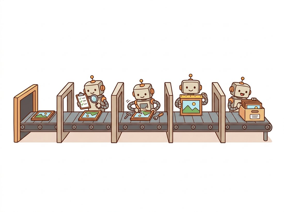
Figure 0.5.1 names the five stages and, more importantly for this book, shows where each one is deepened later. Reading pipelines as instances of this template is a transferable skill: when you meet a training data loader in Chapter 21 or an evaluation harness for generated images in Part IV, you will recognize the same five boxes wearing different costumes.

Two of the five boxes are routinely skipped by beginners and never by professionals: validate (the contract checks of Section 0.4) and measure. Measurement is what turns "the output looks fine" into "mean brightness 131.4, foreground coverage 23.7 percent, PSNR versus original 31.2 dB", numbers that can be logged, compared across versions, and alarmed on. Pipelines fail at the seams, and numbers at the seams are how you notice.

2. The Pipeline, Top to Bottom Beginner

We build the system in three fragments: helpers, metrics, and the orchestrating main. Together they form one runnable script of about ninety lines. The task: convert to grayscale, suppress sensor noise with a light Gaussian blur, segment the bright foreground with Otsu's automatic threshold (previewing Chapter 2), and report what happened. So that the script runs anywhere, it synthesizes a test scene if no input path is given; with an argument, it processes your photo instead.

"""first_pipeline.py: load, validate, transform, measure, save."""
from pathlib import Path
import json, sys, time
import numpy as np
import cv2

def synthesize_scene(h=480, w=640, seed=0) -> np.ndarray:
    """A synthetic 'photo': dark background, bright blobs, sensor noise."""
    rng = np.random.default_rng(seed)
    img = np.full((h, w), 60, np.float32)               # dark background
    for _ in range(6):                                   # bright elliptical blobs
        cy, cx = rng.integers(60, h-60), rng.integers(80, w-80)
        axes = (int(rng.integers(25, 70)), int(rng.integers(20, 50)))
        cv2.ellipse(img, (cx, cy), axes, float(rng.uniform(0, 180)),
                    0, 360, float(rng.uniform(170, 230)), -1)
    img += rng.normal(0, 10, (h, w)).astype(np.float32)  # additive noise
    bgr = cv2.cvtColor(img.clip(0, 255).astype(np.uint8), cv2.COLOR_GRAY2BGR)
    return bgr

def load_validated(path: str | None) -> np.ndarray:
    """Stage 1 + 2: read (or synthesize) and check the contract."""
    if path is None:
        img = synthesize_scene()
    else:
        img = cv2.imread(path, cv2.IMREAD_COLOR)        # uint8 BGR by contract
        if img is None:
            raise ValueError(f"Could not read image: {path}")
    assert img.ndim == 3 and img.dtype == np.uint8, (img.shape, img.dtype)
    return img

Next, the transform and measure stages. The transform is three calls; the interesting choices are in the measurement. We record simple statistics, the automatically chosen threshold, the fraction of pixels classified as foreground, and the peak signal-to-noise ratio between the original grayscale and its blurred version, quantifying exactly how much the blur changed the image. PSNR is defined from mean squared error,

$$\mathrm{MSE} = \frac{1}{HW}\sum_{y=0}^{H-1}\sum_{x=0}^{W-1}\bigl(I(y,x) - K(y,x)\bigr)^2, \qquad \mathrm{PSNR} = 10\,\log_{10}\!\frac{255^2}{\mathrm{MSE}},$$

measured in decibels; higher means more similar, with identical images at infinity. It is the first member of an evaluation lineage this book follows all the way to FID in Chapter 37.

def psnr(a: np.ndarray, b: np.ndarray) -> float:
    """Peak signal-to-noise ratio between two same-shape uint8 images, in dB."""
    mse = np.mean((a.astype(np.float64) - b.astype(np.float64)) ** 2)
    return float("inf") if mse == 0 else 10 * np.log10(255.0 ** 2 / mse)

def transform_and_measure(bgr: np.ndarray) -> tuple[dict, dict]:
    """Stages 3 + 4: grayscale, denoise, segment; measure every product."""
    gray    = cv2.cvtColor(bgr, cv2.COLOR_BGR2GRAY)
    blurred = cv2.GaussianBlur(gray, (5, 5), 1.2)
    t, mask = cv2.threshold(blurred, 0, 255,
                            cv2.THRESH_BINARY + cv2.THRESH_OTSU)
    images = {"gray": gray, "blurred": blurred, "mask": mask}
    metrics = {
        "mean_brightness": round(float(gray.mean()), 2),
        "std_brightness":  round(float(gray.std()), 2),
        "otsu_threshold":  float(t),
        "foreground_frac": round(float((mask > 0).mean()), 4),
        "psnr_blur_db":    round(psnr(gray, blurred), 2),
    }
    return images, metrics

Finally, persistence. The pixels go out as lossless PNGs (Section 0.3 explained why not JPEG for intermediate products), and the numbers go into a JSON sidecar together with the input identity, parameters, library versions, and a timestamp, everything a colleague, or you in six months, needs to trust and reproduce the run.

def save_results(images: dict, metrics: dict, outdir="results") -> Path:
    """Stage 5: lossless pixels plus a JSON sidecar of metrics and context."""
    out = Path(outdir); out.mkdir(exist_ok=True)
    for name, img in images.items():
        ok = cv2.imwrite(str(out / f"{name}.png"), img)
        assert ok, f"imwrite failed for {name}"
    sidecar = {
        "metrics": metrics,
        "params":  {"blur_ksize": 5, "blur_sigma": 1.2, "method": "otsu"},
        "env":     {"opencv": cv2.__version__, "numpy": np.__version__},
        "created": time.strftime("%Y-%m-%dT%H:%M:%S"),
    }
    (out / "run.json").write_text(json.dumps(sidecar, indent=2))
    return out

if __name__ == "__main__":
    src = sys.argv[1] if len(sys.argv) > 1 else None
    images, metrics = transform_and_measure(load_validated(src))
    where = save_results(images, metrics)
    print(json.dumps(metrics, indent=2), "\nsaved to:", where.resolve())

# $ python first_pipeline.py
# {
#   "mean_brightness": 78.66,
#   "std_brightness": 45.21,
#   "otsu_threshold": 121.0,
#   "foreground_frac": 0.1373,
#   "psnr_blur_db": 36.13
# }
# saved to: .../results        (exact values vary slightly per platform)

3. Reading the Numbers Intermediate

Run the script a few times with different seeds and watch the metrics move; this is the cheapest intuition-building exercise in the chapter. The Otsu threshold lands between the background level (around 60) and the blob brightnesses (170 to 230), exactly where a histogram of the scene has its valley, an idea Chapter 2 develops into a complete theory of automatic thresholding. The PSNR of the blur, in the mid-30s of decibels, quantifies "gentle smoothing": strong enough to suppress the $\sigma = 10$ sensor noise, weak enough to keep edges. And the foreground fraction is the pipeline's actual product, the number a downstream consumer would chart over time.

from skimage.metrics import peak_signal_noise_ratio, structural_similarity

p = peak_signal_noise_ratio(gray, blurred)                  # dtype-aware peak
s = structural_similarity(gray, blurred)                    # full SSIM machinery

4. The Same Skeleton, All the Way Up Beginner

It is worth saying explicitly how far this skeleton travels, because the claim sounds immodest for ninety lines of code. Replace the transform stage with learned convolutions and the measure stage with mAP, and you have the object detectors of Chapter 23; modern frameworks such as Ultralytics' YOLO models hide exactly this load-validate-transform-measure-save loop, letterboxing included, behind a one-line API. Replace the transform with iterative denoising and the measure with FID, and you have the evaluation loop of a diffusion model. The boxes get extraordinarily smarter; the seams, and the discipline at the seams, are the constant. That constancy is also why the defensive habits of Section 0.4 were worth a whole section: they apply verbatim at every scale.

5. Chapter Coda: What You Can Now Do Beginner

You can describe any image by shape, dtype, range, and channel order; choose the right library for a job and convert at boundaries; move images in and out of files without losing bits you meant to keep; recognize the four convention clashes on sight; and assemble the five-stage skeleton with measurement built in. That is the entire foundation this book asks for. Chapter 1 now rewinds to the moment before imread: how light becomes the array in the first place, and why its values, resolution, and colors are what they are.