Brightness, Contrast & Gamma Correction

"They told me to brighten up. So I added 50 to everything and clipped my feelings at 255."

A Chronically Underexposed Security Camera

In Chapter 1 we followed light from photons to a quantized grid of numbers, and in Chapter 0 we learned to hold that grid as a NumPy array without mangling its dtype. Until now, though, we have only loaded, inspected, and converted images. This section is where we change one for the first time. We start with the gentlest possible change: transformations that look at a single pixel value and replace it with another, with no knowledge of any neighboring pixel. The restriction sounds severe, yet it covers nearly every exposure and tone adjustment performed in practice.

1. Point Operations: One Pixel In, One Pixel Out Basic

Formally, a point operation (also called an intensity transformation) maps an input image $f$ to an output image $g$ via a function $T$ that depends only on the pixel's own value:

$$g(x, y) = T\big(f(x, y)\big)$$

The coordinates $(x, y)$ appear on both sides but $T$ itself ignores them: the same function is applied at every location. Contrast this with the neighborhood operations of Chapter 3, where the output at $(x,y)$ depends on a whole window of surrounding pixels. The independence of point operations has three practical consequences. First, they are trivially parallel: every pixel can be processed at once, which is why they vectorize perfectly in NumPy and run essentially for free on a GPU. Second, they can never sharpen, blur, or denoise, because those effects require comparing neighbors. Third, for 8-bit images, any point operation whatsoever can be precomputed as a table of 256 output values, a fact we will exploit shortly.

Because $T$ maps the interval $[0, 255]$ to itself, we can draw it: input intensity on the horizontal axis, output intensity on the vertical. Figure 2.1.1 plots the transfer curves of the four operations this section covers. The identity is the diagonal; brightness shifts the diagonal up; contrast rotates it steeper around a pivot; gamma bends it into a power-law curve. Reading transfer curves fluently is a genuinely useful skill: it is exactly how photographers read the "curves" panel, and how you will debug a mysterious tone shift in a data pipeline.

2. Brightness and Contrast: The Linear Family Basic

The workhorse point operation is affine:

$$g(x, y) = \alpha \cdot f(x, y) + \beta$$

where $\alpha$ (the gain) controls contrast and $\beta$ (the bias) controls brightness. With $\alpha > 1$ the intensity range stretches and the image looks punchier; with $\alpha < 1$ it compresses and the image looks flat. Positive $\beta$ lifts everything toward white. The subtlety is not the formula but the arithmetic around it: the result $\alpha r + \beta$ routinely lands outside $[0, 255]$, and as we saw when discussing dtypes in Chapter 0, uint8 arithmetic wraps around rather than saturating. The from-scratch implementation below does it correctly: compute in float, clip, then convert back.

import numpy as np
import cv2

img = cv2.imread("scene.jpg")          # uint8 BGR, shape (H, W, 3)

def adjust_brightness_contrast(img, alpha=1.0, beta=0):
    """Apply g = alpha * f + beta with correct saturation."""
    out = img.astype(np.float32) * alpha + beta   # work in float32: no overflow
    out = np.clip(out, 0, 255)                    # saturate instead of wrapping
    return out.astype(np.uint8)                   # back to displayable uint8

punchy = adjust_brightness_contrast(img, alpha=1.3, beta=-20)
washed = adjust_brightness_contrast(img, alpha=0.6, beta=80)

print(img[0, 0], "->", punchy[0, 0])
# Example output for a pixel [200 180 90]:
# [200 180 90] -> [240 214 97]   (the 200 channel hit 240 = 1.3*200 - 20)

The function above is six lines. OpenCV collapses it to one, and handles the saturation internally with optimized SIMD code. Whenever you see yourself writing the float-clip-convert dance for an affine adjustment, reach for the library instead.

punchy = cv2.convertScaleAbs(img, alpha=1.3, beta=-20)

3. Gamma Correction: The Power-Law Curve Intermediate

Linear adjustments move all intensities by the same recipe, but human vision does not work linearly: we are far more sensitive to differences in shadows than in highlights. As covered in Chapter 1, this is why almost every stored image is gamma-encoded: the camera applies a power law that allocates more of the 256 code values to darker tones, and the display applies the inverse. The same power law, applied deliberately, is the standard tool for tonal correction. On intensities normalized to $[0, 1]$:

$$s = r^{\gamma}$$

With $\gamma < 1$ the curve bows upward and shadows brighten dramatically while highlights barely move (the red curve in Figure 2.1.1). With $\gamma > 1$ the curve bows downward and the image darkens, with midtones affected most (the orange curve). Because the endpoints 0 and 1 map to themselves, gamma never clips: it redistributes the tonal range instead of truncating it, which is exactly why it is preferred over a brightness shift for fixing exposure.

import numpy as np
import cv2

def gamma_correct(img, gamma):
    """Apply s = r**gamma on normalized intensities via a 256-entry LUT."""
    r = np.arange(256, dtype=np.float32) / 255.0   # all possible inputs, normalized
    table = np.clip(255.0 * (r ** gamma), 0, 255).astype(np.uint8)
    return cv2.LUT(img, table)                     # one table lookup per pixel

img = cv2.imread("underexposed_loading_dock.jpg")
brighter = gamma_correct(img, gamma=0.5)   # gamma < 1 lifts shadows
darker   = gamma_correct(img, gamma=2.0)   # gamma > 1 deepens them

# Spot-check the curve itself:
print(int(255 * (50/255) ** 0.5))    # 112  : deep shadow 50 jumps to 112
print(int(255 * (200/255) ** 0.5))   # 225  : highlight 200 moves only to 225

Note what the code does: rather than computing img ** gamma over the whole array (millions of float power operations), it evaluates the curve at the 256 possible uint8 values and lets cv2.LUT do a table lookup per pixel. The spot-check printout confirms the asymmetry that makes gamma so useful: an input of 50 jumps to 112, while 200 only creeps to 225. If you work in PyTorch data pipelines, the equivalent is torchvision.transforms.v2.functional.adjust_gamma, and randomized gamma is a standard photometric augmentation we will meet again in Chapter 21.

4. Lookup Tables: Point Operations at Production Speed Intermediate

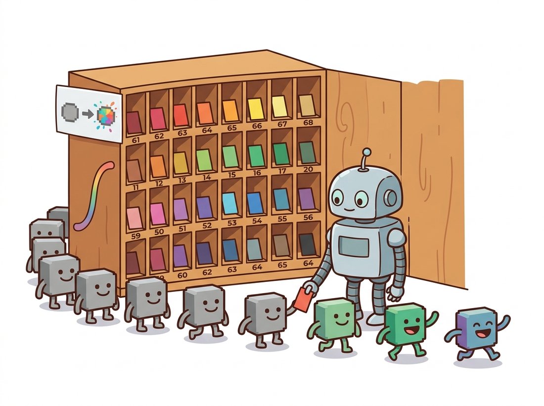
The gamma example quietly introduced the most important implementation idea of this section: for 8-bit data there are only 256 possible input values, so any point operation, however expensive its formula, costs exactly 256 function evaluations plus one table lookup per pixel. Better still, lookup tables compose. If you want to apply contrast, then gamma, then a tone tweak, you do not run three passes over the image; you compose the three curves into one table and run a single pass. This is precisely how camera ISPs, video pipelines, and color-grading systems work internally, and it is why colorists exchange ".cube" LUT files rather than scripts.

import numpy as np
import cv2

def build_tone_lut(alpha=1.0, beta=0.0, gamma=1.0):
    """Compose contrast/brightness and gamma into ONE 256-entry table."""
    r = np.arange(256, dtype=np.float32)
    r = np.clip(alpha * r + beta, 0, 255) / 255.0   # stage 1: affine
    s = np.clip(255.0 * (r ** gamma), 0, 255)       # stage 2: gamma
    return s.astype(np.uint8)

lut = build_tone_lut(alpha=1.2, beta=-10, gamma=0.8)

cap = cv2.VideoCapture("dock_camera.mp4")
while True:
    ok, frame = cap.read()
    if not ok:
        break
    corrected = cv2.LUT(frame, lut)    # entire tone pipeline: one lookup pass
    # ... feed `corrected` to the detector ...

The pattern in this code, build the table once and reuse it for every frame, is worth internalizing. It converts per-pixel math into per-codebook math, and it scales to color: a 3D LUT tabulates a function of (R, G, B) jointly on a coarse lattice and interpolates between entries, which is how film looks and display calibration are implemented. Keep this in mind when you reach learned enhancement later: several state-of-the-art methods literally predict LUTs.

5. Choosing Parameters Automatically: Percentile Stretching Intermediate

Everything so far required a human to pick $\alpha$, $\beta$, or $\gamma$. A first step toward automation is contrast stretching: map the darkest interesting intensity to 0 and the brightest to 255, linearly. Using the absolute minimum and maximum is fragile (one dead pixel ruins the stretch), so robust implementations use percentiles, typically the 2nd and 98th:

$$g = 255 \cdot \frac{\mathrm{clip}(f,\, p_2,\, p_{98}) - p_2}{p_{98} - p_2}$$

import numpy as np

def autocontrast(gray, low_pct=2, high_pct=98):
    """Percentile-based contrast stretch (robust to outlier pixels)."""
    lo, hi = np.percentile(gray, [low_pct, high_pct])
    if hi <= lo:                       # flat image: nothing to stretch
        return gray.copy()
    out = (gray.astype(np.float32) - lo) * (255.0 / (hi - lo))
    return np.clip(out, 0, 255).astype(np.uint8)

# A hazy image occupying only [90, 170] gets remapped to use [0, 255]:
hazy = np.random.randint(90, 171, size=(480, 640), dtype=np.uint8)
stretched = autocontrast(hazy)
print(hazy.min(), hazy.max(), "->", stretched.min(), stretched.max())
# 90 170 -> 0 255

Notice what autocontrast needed in order to act: the percentiles of the intensity distribution. We computed them directly here, but the principled tool for describing that distribution is the histogram, and once you have a histogram you can do far more than stretch endpoints: you can diagnose exposure problems, compare images, and derive optimal contrast curves and thresholds. That is the subject of the next two sections, beginning with Section 2.2.