The Sampling Theorem, Aliasing & Anti-Aliasing

"They photographed me at two pixels per plank and now the internet thinks I'm a rainbow. I am a fence. I have always been a fence."

An Undersampled Picket Fence

Section 4.3 sculpted spectra deliberately. This section is about the spectral surgery you perform by accident every time you shrink an image. Resizing feels like an innocent operation, yet it is the most common way real pipelines corrupt their data, and the corruption has a special property that makes it dangerous: it is invisible in code review, intermittent in testing (it depends on image content), and irreversible once it happens. The frequency view from this chapter makes the mechanism, and therefore the cure, completely transparent.

1. Sampling Through the Frequency Lens Intermediate

Mathematically, sampling a continuous signal means multiplying it by a train of impulses spaced $1/f_s$ apart, where $f_s$ is the sampling rate. The frequency-domain consequence is the key to everything: multiplication by an impulse train in space equals convolution with an impulse train in frequency, so the sampled signal's spectrum is the original spectrum copied over and over, with replicas centered at every multiple of $f_s$:

$$F_s(u) \;=\; f_s \sum_{k=-\infty}^{\infty} F(u - k f_s)$$

Reconstruction means isolating the central copy with a low-pass filter. That works precisely when the copies do not touch, and the copies do not touch precisely when the original spectrum ends before the next replica begins: $f_s > 2 f_{\max}$, the Nyquist criterion. Made concrete: a pixel grid samples once per pixel, so its sampling rate is 1 cycle per pixel, and the finest pattern it can hold is therefore 0.5 cycles per pixel (one full light-dark cycle every two pixels). Anything finer than that half-cycle limit will alias. Figure 4.4.1 tells the whole story in two rows. When the criterion fails, neighboring replicas overlap, their tails add irreversibly, and a frequency $f$ above the limit masquerades as the lower frequency $|f - k f_s|$ folded back into range. That impostor is an alias.

A single arithmetic line makes the masquerade concrete. Sample at $f_s = 1$ cycle per pixel (one sample per pixel, so the Nyquist limit is $0.5$). A genuine pattern at $f = 0.4$ cycles per pixel sits safely under the limit and is recorded faithfully. But a finer pattern at $f = 0.7$ cycles per pixel exceeds the limit, so it folds: $|0.7 - 1| = 0.3$ cycles per pixel. The sensor cannot tell that $0.7$ apart from a true $0.3$ pattern; both produce identical samples, and the recorded image shows a coarse $0.3$ stripe where the scene had a fine $0.7$ one.

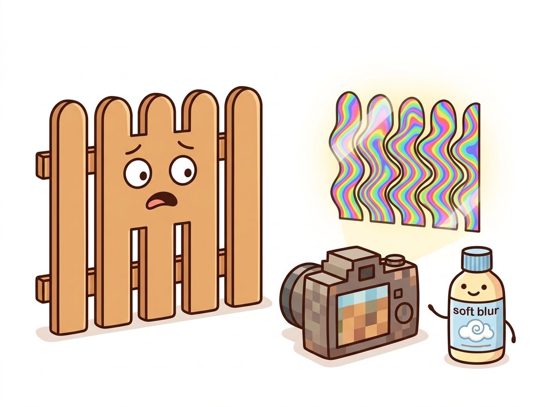
One more example fixes the pattern in mind. Push the input to $f = 0.9$ and it folds to $|0.9 - 1| = 0.1$: the finer the unrepresentable detail, the coarser and more conspicuous the lie it leaves behind. That is exactly why a tightly woven fabric photographed too small turns into broad swirling bands rather than simply disappearing.

2. Seeing Aliasing: The Zone Plate Torture Test Beginner

The standard instrument for catching resamplers misbehaving is the zone plate: concentric rings whose frequency grows linearly with radius, sweeping from zero at the center to the Nyquist limit at the edge. Any aliasing shows up as ghostly secondary ring families blooming where no rings should be. The test costs five lines:

# Build a zone plate (rings whose frequency grows with radius) and shrink it
# three ways: bare decimation, OpenCV's INTER_AREA, and an explicit Gaussian
# prefilter. Only the prefiltered routes remove unrepresentable detail first.
import numpy as np
import cv2

N = 512
yy, xx = np.mgrid[0:N, 0:N].astype(np.float64)
r2 = (xx - N / 2) ** 2 + (yy - N / 2) ** 2
zone = np.cos(np.pi * r2 / N)         # radial frequency grows linearly with radius

factor = 4
naive = zone[::factor, ::factor]      # decimation, no prefilter: aliasing factory
area  = cv2.resize(zone, (N // factor, N // factor),
                   interpolation=cv2.INTER_AREA)          # box prefilter built in
sigma = 0.5 * factor                  # blur matched to the reduction factor
prefiltered = cv2.GaussianBlur(zone, (0, 0), sigmaX=sigma)[::factor, ::factor]

# naive: loud families of false rings swirl across the whole image.
# area and prefiltered: the true central rings, fading smoothly to flat
# gray where frequencies above the new Nyquist limit were removed.

Display the three results and the lesson is unforgettable: the naive decimation does not merely lose the fine outer rings, it invents coarse rings that were never there. This is exactly the moiré you have seen photographing a window screen, a fine-knit sweater, or a distant roof of tiles, and it is also why the rotating wagon wheels of old westerns spin backward: film at 24 frames per second is temporal sampling, and a wheel spoke passing faster than 12 cycles per second folds back into apparent slow or reverse rotation. The illustration below tells the same cautionary tale: shrink a fine pattern without blurring first and the sampler invents coarse rainbows that were never there.

3. Anti-Aliasing Done Right Intermediate

The universal recipe is prefilter, then sample: reduce the image's bandwidth to fit the new sampling rate, then decimate. The five-word version, worth taping above any resize call, is in the tip below. For a reduction by factor $s$, the new Nyquist limit is $1/s$ of the old one, so the prefilter must suppress everything above it; for the Gaussian prefilter of Chapter 3, $\sigma \approx 0.5 s$ is a serviceable rule of thumb (scikit-image's resize uses the close cousin $\sigma = (s - 1)/2$ when its anti-aliasing is enabled). What trips teams up is that common APIs distribute this responsibility unevenly. In OpenCV, INTER_AREA averages over the source footprint and is the correct flag for shrinking, while INTER_LINEAR and INTER_NEAREST sample only a tiny neighborhood and alias badly at large reductions (they are interpolators, designed for enlarging, where the considerations are different and which Chapter 5 treats in depth). PyTorch carries the same hazard, as the code below shows once we have the recipe in hand.

That recipe carries straight into the deep learning stack, where the default behavior is the trap. In PyTorch, F.interpolate aliases by default and anti-aliasing is opt-in, so the code below runs the zone-plate shrink both ways to expose the difference one flag makes:

# Repeat the downsampling experiment inside PyTorch to show that antialiasing
# is opt-in: F.interpolate aliases by default, and antialias=True is the entire
# difference between fabricated ghost rings and a correctly bandlimited result.
import torch
import torch.nn.functional as F

t = torch.from_numpy(zone)[None, None]                  # (1, 1, 512, 512)
no_aa = F.interpolate(t, scale_factor=0.25, mode="bilinear")
aa    = F.interpolate(t, scale_factor=0.25, mode="bilinear", antialias=True)

# no_aa reproduces the naive ghost rings on the GPU; aa widens the
# bilinear kernel to cover the full source footprint and matches the
# clean result of Code 4.4.1.

from torchvision.transforms import v2
small = v2.Resize(128, antialias=True)(t)    # antialias defaults to True in v2

4. Aliasing Inside Neural Networks Advanced

The sampling theorem does not stop applying when the pixels enter a network. Every stride-2 convolution and every pooling layer in the CNNs of Chapter 19 is a downsampling step, and most classic architectures perform it with no adequate prefilter. Max pooling is particularly lawless, since taking a maximum is not even linear, let alone bandlimited. The measurable symptom is broken shift invariance: shift the input image by a single pixel and a classifier's confidence can swing dramatically, because aliased feature maps fold the shift into spurious low-frequency changes.

Three landmark fixes all apply this chapter's recipe inside the network. Richard Zhang's BlurPool (ICML 2019) inserts a small fixed blur before each stride and improves both shift stability and plain accuracy across architectures. StyleGAN3 (NeurIPS 2021) pushed the discipline through an entire generator, treating every feature map as a continuous bandlimited signal with carefully matched filters at each resampling, which cured the eerie "texture sticking" of earlier GANs where hair and skin detail stayed glued to screen coordinates while faces moved. Alias-Free Convnets (CVPR 2023) extended the program to full fractional-shift equivariance in classifiers, taming the nonlinearities that reintroduce high frequencies.