Image Pyramids: Gaussian & Laplacian

"Every floor of my building is a quarter the size of the one below, nobody can explain where the lost square footage went, and yet from the penthouse you can still reconstruct the lobby exactly. Real estate hates this one trick."

A Vertigo-Prone Image Pyramid

Section 4.4 taught the safe way to halve an image: blur away the unrepresentable frequencies, then decimate. Do that once and you have a thumbnail; do it repeatedly, keeping every intermediate, and you have a Gaussian pyramid, a data structure so useful that Burt and Adelson's 1983 paper introducing its Laplacian refinement remains one of the most cited works in image processing. This section builds both pyramids from parts you already own, proves the Laplacian's perfect-reconstruction property in code, and closes with the trick that made the construction famous: blending two images so seamlessly that the seam cannot be found.

1. Why Multi-Scale? Beginner

Image content does not live at one scale. A face fills 400 pixels in a portrait and 12 pixels in a group photo; the same crosswalk is a texture from a drone and an obstacle from a bumper camera. Any algorithm with a fixed receptive footprint, a correlation template, a corner detector, a convolution kernel from Chapter 3, is therefore tuned to one band of object sizes and blind outside it. The multi-scale answer is disarmingly literal: run the algorithm at many resolutions of the same image. Small templates on coarse levels find large objects; the same templates on fine levels find small ones. Coarse-to-fine search adds a second gift: solve the problem cheaply on a tiny level, then refine the answer down the ladder, touching only a neighborhood at each finer level. Registration, stereo, optical flow, and template matching all exploit this schedule, and you will meet it again as the scale space inside SIFT in Chapter 10.

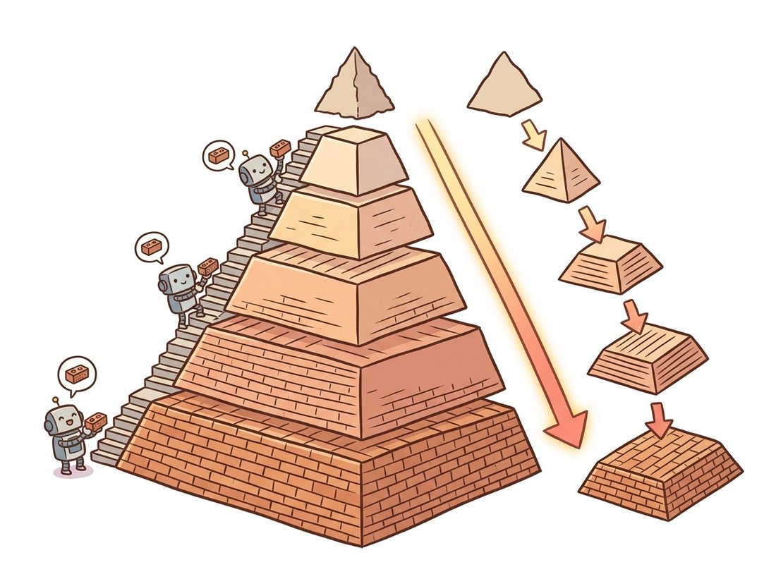
2. The Gaussian Pyramid: REDUCE, Repeated Beginner

One pyramid step is the REDUCE operation: convolve with a small low-pass kernel $w$, then keep every second pixel in each direction,

$$G_{k+1} = \big(w * G_k\big)\downarrow_2, \qquad G_0 = \text{the original image}$$

Burt and Adelson's classic $w$ is the 5-tap binomial kernel $\tfrac{1}{16}[1, 4, 6, 4, 1]$ applied separably, a snug approximation to the Gaussian prefilter that Section 4.4 demands before 2x decimation. OpenCV packages the whole step as cv2.pyrDown:

import numpy as np
import cv2
from skimage import data

img = data.astronaut()                      # 512 x 512 x 3, uint8

def gaussian_pyramid(image, levels):
    pyr = [image]
    for _ in range(levels - 1):
        pyr.append(cv2.pyrDown(pyr[-1]))    # blur with [1,4,6,4,1]/16, then halve
    return pyr

gp = gaussian_pyramid(img, levels=5)
print([level.shape[:2] for level in gp])
# [(512, 512), (256, 256), (128, 128), (64, 64), (32, 32)]
# Total storage: 1 + 1/4 + 1/16 + ... < 4/3 of the original image.

Each level of the result answers a different question. $G_0$ holds everything; $G_2$ holds what survives viewing from four times the distance; $G_4$ holds only the broad strokes of the composition. What the Gaussian pyramid does not tell you is what each level lost, and that observation is the doorway to the second construction.

3. The Laplacian Pyramid: Storing the Differences Intermediate

Define EXPAND as the upsampling twin of REDUCE (insert zeros, interpolate with the same kernel; cv2.pyrUp). Then each Laplacian level is what a Gaussian level contains beyond what its coarser neighbor can explain:

$$L_k = G_k - \text{EXPAND}(G_{k+1}), \qquad L_{\text{top}} = G_{\text{top}}$$

Each $L_k$ is a band-pass image: it holds the detail in one octave of spatial frequency, the band that lives between level $k$'s resolution and level $k{+}1$'s. (It is the discrete sibling of the difference-of-Gaussians band-pass from Chapter 3, which is why the name honors the Laplacian operator.) The construction is trivially invertible by running it backward, $G_k = L_k + \text{EXPAND}(G_{k+1})$, so the pyramid of differences plus the tiny top level is a complete, perfectly reconstructable code for the image. Figure 4.5.1 lays out both directions.

def laplacian_pyramid(image, levels):
    gp = gaussian_pyramid(image.astype(np.float32), levels)
    lp = []
    for i in range(levels - 1):
        up = cv2.pyrUp(gp[i + 1], dstsize=gp[i].shape[1::-1])  # EXPAND to (w, h)
        lp.append(gp[i] - up)                                  # one octave of detail
    lp.append(gp[-1])                                          # coarse residual on top
    return lp

def reconstruct(lp):
    out = lp[-1]
    for lap in reversed(lp[:-1]):
        out = cv2.pyrUp(out, dstsize=lap.shape[1::-1]) + lap
    return out

lp = laplacian_pyramid(img, levels=5)
restored = reconstruct(lp)
print(np.abs(restored - img.astype(np.float32)).max())   # 0.0 (exact in float32)

4. Multi-Band Blending: The Trick That Made Pyramids Famous Intermediate

Paste two photos along a seam and your eye finds the cut instantly. Feather them with a wide alpha ramp and the seam blurs into a ghostly band instead. The diagnosis is spectral: a transition's correct width depends on wavelength. Coarse content (lighting, sky tone) should blend over a wide region; fine content (grass blades, fabric) should hand over within pixels. No single-width blend can satisfy both, but a pyramid blends every octave at its own natural width: decompose both images into Laplacian pyramids, blend each level under a Gaussian-pyramid-smoothed mask, and reconstruct.

def multiband_blend(a, b, mask, levels=6):
    """mask: float image in [0,1]; 1 keeps a, 0 keeps b."""
    la = laplacian_pyramid(a, levels)
    lb = laplacian_pyramid(b, levels)
    gm = gaussian_pyramid(mask.astype(np.float32), levels)
    blended = [m * x + (1.0 - m) * y for x, y, m in zip(la, lb, gm)]
    return np.clip(reconstruct(blended), 0, 255).astype(np.uint8)

a_img = data.astronaut().astype(np.float32)                  # 512 x 512 x 3
b_img = cv2.resize(data.coffee(), (512, 512)).astype(np.float32)

mask = np.zeros(a_img.shape[:2], np.float32)
mask[:, : a_img.shape[1] // 2] = 1.0          # hard left/right split
mask = mask[..., None].repeat(3, axis=2)      # broadcast over color channels

seamless = multiband_blend(a_img, b_img, mask)
# The hard mask edge is smoothed differently at every level: wide for
# coarse bands, narrow for fine bands. The two photos fuse with no
# visible seam, the same trick as Burt and Adelson's famous orapple.

from skimage.transform import pyramid_gaussian, pyramid_laplacian
gp = list(pyramid_gaussian(img, max_layer=4, channel_axis=-1))   # one line
lp = list(pyramid_laplacian(img, max_layer=4, channel_axis=-1))  # one line

blender = cv2.detail_MultiBandBlender(num_bands=5)   # production blending

5. The Pyramid's Afterlife in Deep Learning Advanced

Squint at a modern vision backbone and you will see this section's diagram. A CNN halves resolution stage by stage while deepening its channels: a learned Gaussian pyramid, with each stage's features playing the role of a level (the architectures of Chapter 20 make the correspondence explicit). Feature Pyramid Networks bolt on a top-down path with lateral connections, adding coarse semantic context back into fine levels, which is EXPAND-and-add wearing learned weights, and FPN-style necks remain standard in the detection and segmentation systems of Chapter 24. The reconstruction direction has an afterlife too: generative models that synthesize coarse structure first and add octaves of detail are running Code 4.5.2's loop with a neural network inside.