Warping, Remapping & Inverse Mapping

"I never ask where a pixel is going. I stand at the destination and ask where it came from. People call it pessimism; I call it complete coverage."

A Contrarian Inverse Mapper

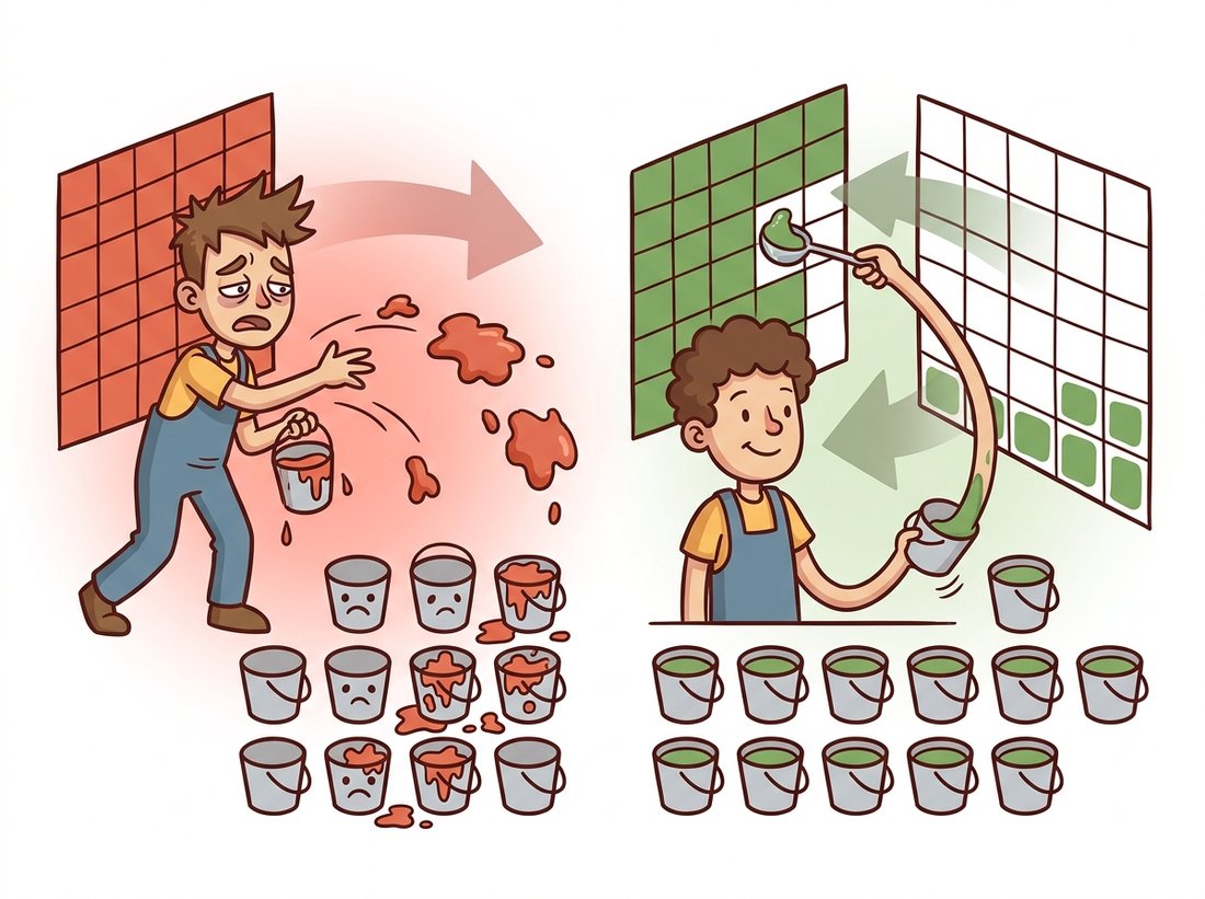
We now hold both halves of the puzzle: Section 5.2 gave us matrices that map coordinates, and Section 5.3 gave us interpolation to read values at the fractional positions those matrices produce. This section assembles them into the actual algorithm that executes a warp, and the assembly contains the chapter's most important engineering idea. It is not obvious, most newcomers implement the wrong version first, and the right version is one line of insight: loop over the output, not the input.

1. Forward Mapping and Why It Fails Intermediate

The intuitive algorithm reads: for each input pixel $(x, y)$, compute its destination $(x', y') = M(x, y)$, round to the nearest grid position, and copy the value there. This is forward mapping (also called splatting), and it has two failure modes that are not edge cases but guarantees. First, holes: under any transform that locally magnifies, neighboring input pixels land more than one pixel apart in the output, leaving destination pixels that no input pixel ever claims. Rotate by 15 degrees and the output is peppered with unwritten black dots. Second, collisions: under local minification, several input pixels round to the same destination and overwrite one another arbitrarily, last-writer-wins, which is both lossy and nondeterministic with parallel execution.

Inverse mapping flips the iteration. For each output pixel $(x', y')$, compute the source location via the inverse transform, $(x, y) = M^{-1}(x', y')$, and interpolate the input there:

Every output pixel is visited exactly once, so there are no holes and no collisions by construction. The fractional source position is exactly what the bilinear sampler from Section 5.3 was built for. The only requirement is an invertible transform, which every family in Section 5.1's hierarchy satisfies. Figure 5.4.1 contrasts the two strategies; it is the diagram to redraw from memory if you remember only one from this chapter.

2. Building warpAffine From Scratch Intermediate

Inverse mapping plus the vectorized bilinear_sample from Section 5.3 yields a complete affine warper in under 20 lines. The only new machinery is generating all output coordinates at once with np.mgrid and pushing them through the inverted matrix in a single einsum:

import numpy as np

def warp_affine_scratch(img, M2x3, out_shape):
    """Inverse-mapping affine warp of a grayscale image.

    M2x3 maps INPUT coords to OUTPUT coords (like cv2.warpAffine).
    """
    H_out, W_out = out_shape
    M3 = np.vstack([M2x3, [0.0, 0.0, 1.0]])     # lift to 3x3
    Minv = np.linalg.inv(M3)                    # output -> input

    ys, xs = np.mgrid[0:H_out, 0:W_out].astype(np.float64)
    ones = np.ones_like(xs)
    dst = np.stack([xs, ys, ones])              # 3 x H x W homogeneous grid

    src = np.einsum('ij,jhw->ihw', Minv, dst)   # apply Minv to every pixel
    src_x, src_y = src[0], src[1]               # affine: w stays 1, no divide

    out = bilinear_sample(img, src_x, src_y)    # Section 5.3's sampler

    # Mask coordinates that fell outside the source image (constant border).
    inside = ((src_x >= 0) & (src_x <= img.shape[1] - 1) &
              (src_y >= 0) & (src_y <= img.shape[0] - 1))
    return np.where(inside, out, 0.0)

Three details in Code 5.4.1 deserve attention. First, the matrix we invert is the input-to-output transform, matching OpenCV's convention; the algorithm itself consumes the output-to-input direction, and APIs differ on which one they want (OpenCV's warpAffine accepts flags=cv2.WARP_INVERSE_MAP to skip the inversion). Second, the einsum applies a single $3 \times 3$ matrix to millions of coordinates with no Python loop; this is the vectorization habit from Chapter 0 doing real work. Third, the inside mask implements the simplest border policy: pixels whose source falls outside the input become black. These are the same border questions you met when convolution kernels hung off the image edge in Chapter 3, and OpenCV reuses the identical flags: BORDER_CONSTANT, BORDER_REPLICATE, BORDER_REFLECT_101, and for tiling warps, BORDER_WRAP.

out = cv2.warpAffine(img, M2x3, (W_out, H_out),
                     flags=cv2.INTER_LINEAR,
                     borderMode=cv2.BORDER_REPLICATE)
out = cv2.warpPerspective(img, H3x3, (W_out, H_out))   # homography version

3. Beyond Matrices: remap and the Lookup-Table View Intermediate

Here is the conceptual jump that makes inverse mapping truly powerful: nothing in the algorithm requires the source coordinates to come from a matrix. Any pair of arrays map_x[y, x] and map_y[y, x], declaring for each output pixel where in the input to look, defines a valid warp. OpenCV exposes exactly this as cv2.remap, and it is the escape hatch for every transform that is not projective: lens distortion, fisheye unwrapping, swirl filters, scanline jitter, and the per-pixel flow fields we will meet in Chapter 15.

The canonical real-world example is radial lens distortion. Real lenses bow straight lines outward (barrel distortion, wide-angle lenses) or inward (pincushion, telephoto). The standard model perturbs each point's distance from the image center: with normalized radius $r$,

where $k_1, k_2$ are lens-specific coefficients (where they come from is the calibration story of Chapter 12). To undistort, we build maps that send each output (clean) pixel to its distorted source position and let remap do the rest:

import cv2
import numpy as np

img = cv2.imread("wide_angle.jpg")
h, w = img.shape[:2]
cx, cy = w / 2.0, h / 2.0
k1, k2 = 0.28, 0.06          # barrel distortion strengths (illustrative)

# For each OUTPUT pixel, where in the distorted input is its color?
ys, xs = np.mgrid[0:h, 0:w].astype(np.float32)
xn = (xs - cx) / cx          # normalize to roughly [-1, 1]
yn = (ys - cy) / cy
r2 = xn**2 + yn**2
factor = 1 + k1 * r2 + k2 * r2**2

map_x = (xn * factor * cx + cx).astype(np.float32)
map_y = (yn * factor * cy + cy).astype(np.float32)

undistorted = cv2.remap(img, map_x, map_y,
                        interpolation=cv2.INTER_LINEAR,
                        borderMode=cv2.BORDER_CONSTANT)

Two performance notes turn this from demo into production. The maps depend only on the lens, not the image, so compute them once and reuse them for every frame of a video stream. And cv2.convertMaps converts the float maps into a fixed-point representation (CV_16SC2) that remap executes significantly faster with identical visual results, a standard trick on embedded hardware.

4. Differentiable Warping: grid_sample Advanced

The same gather-and-interpolate operation lives inside PyTorch as torch.nn.functional.grid_sample, with one crucial addition: it is differentiable. Bilinear interpolation is a little weighted sum, so gradients flow through the weights to the sampling coordinates themselves, which means a network can learn where to look. This was the breakthrough of Spatial Transformer Networks (Jaderberg et al., 2015), and it is now plumbing inside registration networks, optical-flow training, and the view-synthesis methods of Chapter 27.

import torch
import torch.nn.functional as F

img_t = torch.rand(1, 3, 240, 320)            # (N, C, H, W)

# grid holds, for each output pixel, the source location in
# NORMALIZED coordinates: x and y each in [-1, 1] over the input.
theta = torch.tensor([[[0.966, -0.259, 0.0],   # 15-degree rotation,
                       [0.259,  0.966, 0.0]]]) # expressed for normalized coords
grid = F.affine_grid(theta, size=img_t.shape, align_corners=False)
warped = F.grid_sample(img_t, grid, mode='bilinear',
                       padding_mode='zeros', align_corners=False)
print(warped.shape)        # torch.Size([1, 3, 240, 320])

The API holds two traps for OpenCV-trained hands. Coordinates are normalized: $(-1, -1)$ is the input's top-left and $(1, 1)$ its bottom-right, so pixel-space maps must be rescaled before use. And the align_corners flag changes what $-1$ and $1$ mean (corner pixel centers versus corner pixel edges); mixing conventions between a model's training code and its deployment code shifts every sample by up to half a pixel, an error small enough to survive code review and large enough to degrade a super-resolution model. Pick align_corners=False (the modern default) and use it everywhere.

5. A Checklist for Production Warps Beginner

Warping code is short but dense with conventions, and most bugs come from the same five questions being answered inconsistently. Before shipping any warp, walk this list:

1. Direction: does your API want the forward matrix or the inverse? (cv2.warp* wants forward and inverts internally; remap and grid_sample consume the inverse-mapped coordinates directly.)
2. Coordinate convention: pixel coordinates or normalized? $(x, y)$ or (row, col)? Size as (width, height) or shape as (height, width)?
3. Interpolation: bilinear for images, nearest for masks and label maps (the phantom-class trap from Section 5.3), and an anti-aliased path if the warp locally minifies.
4. Border policy: what value do out-of-source pixels take, and will downstream code mistake it for content? (A black border feeding a histogram skews it; recall the border discussions of Chapter 3.)
5. Reuse: if the geometry is fixed, are the maps precomputed and fixed-point converted?

With execution machinery in hand, one question remains open, and it is the big one: where do the transforms come from when no one hands you a matrix? Estimating them from the images themselves is image registration, the subject of Section 5.5.