"Half of my data points could be lying to me. Fortunately, I only need four that tell the truth, and I am prepared to keep drawing straws all night."
A Patiently Skeptical Robust Estimator
When data contains outright lies, do not fit a model to all of it; fit many candidate models to the smallest possible random samples and crown the one that the most data agrees with. That inversion is RANSAC, the algorithm that closes this chapter's pipeline. Detection (Section 10.1) found repeatable points, description (Sections 10.3 and 10.4) made them comparable, matching (Section 10.5) produced correspondences that are mostly right, and RANSAC delivers the final product: a geometric model plus a verdict on every single match. Those verified correspondences are what Chapter 12 calibrates cameras with, what Chapter 13 turns into depth, and what Chapter 14 reconstructs cities from.
In the previous section, every filter judged matches one at a time, and the closing admission was that some confidently wrong matches survive any per-match test. This section brings in the judge that per-match filters cannot replace: geometry. All true correspondences between two views of a rigid scene are bound by a single global model (a homography for planar scenes, a fundamental matrix in general), while false matches scatter without pattern. Fitting that model to contaminated data, and using the fit to separate inliers from outliers, is the problem of robust estimation, and the 1981 algorithm that solves it remains one of the most-used tools in all of computer vision.
1. The Tyranny of the Squared Residual Beginner
Start with the failure. Suppose you have $n$ matched point pairs and want the line (or homography, the logic is identical) that best explains them. The instinct trained by every statistics course is least squares: choose the model parameters that minimize $\sum_i r_i^2$, the sum of squared residuals. Least squares is optimal when residuals are well-behaved Gaussian noise, and the fits of Chapter 9 leaned on it happily. But a false match is not noise. A correct SIFT match might be off by half a pixel; a false match connecting a roof corner to a fence post is off by four hundred pixels, and the square of its residual is 640,000 times larger than the square of a correct match's. Minimizing the sum, the model abandons a hundred honest points to appease one liar. Statisticians say least squares has a breakdown point of zero: a single sufficiently bad outlier corrupts the fit by an arbitrary amount. The tug-of-war below shows how one loud liar drags the naive fit while the robust fit fences the liars out.
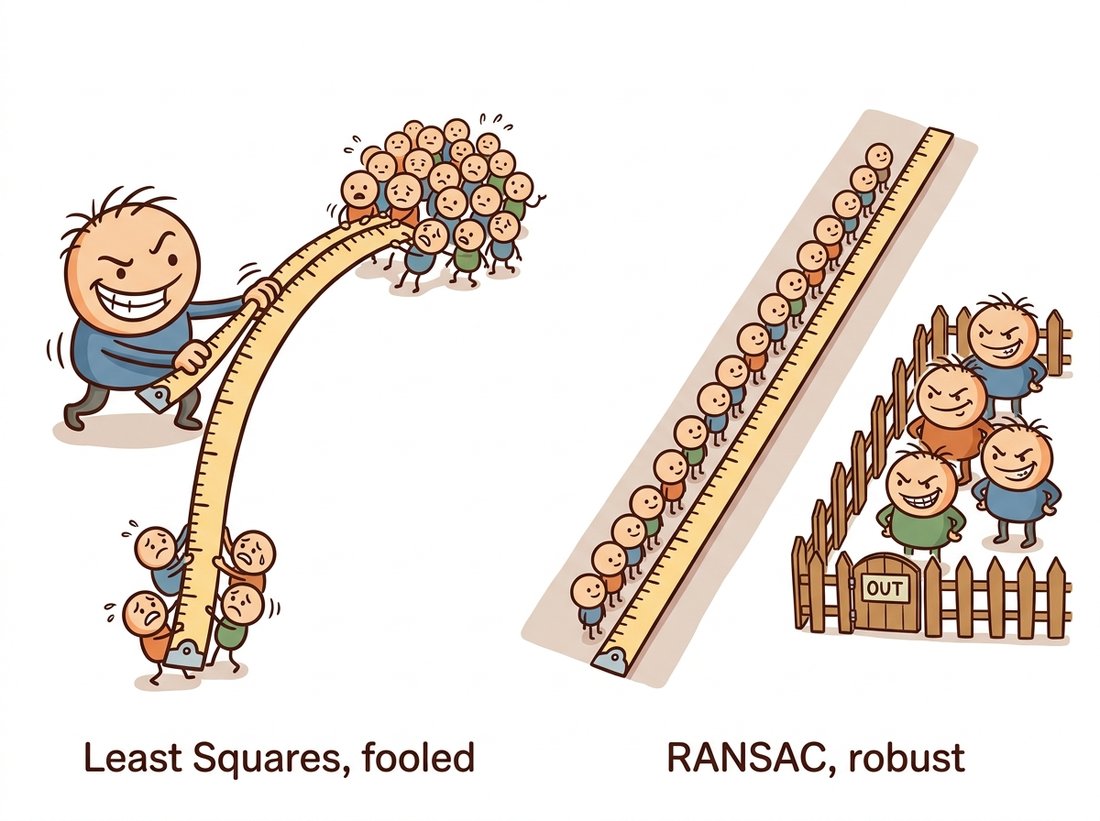
Figure 10.6.1 shows the disease and the cure on the simplest possible model. On the left, a handful of outliers drags the least-squares line off the obvious trend; the fit serves nobody, neither the inliers nor the outliers. On the right, the RANSAC fit ignores the outliers entirely, recovering the line the inliers define, with a tolerance band that makes the inlier-or-outlier verdict explicit. Nothing about the picture changes when the model becomes a homography with eight parameters instead of a line with two; only the minimal sample size grows.
Readers of Chapter 9 have already met one cure for outliers: the Hough transform, where every edge pixel votes for all the lines through it and real lines emerge as peaks no minority can suppress. RANSAC is the Hough idea run in the opposite direction. Hough discretizes parameter space and lets data vote in it, which works beautifully for two or three parameters and dies of memory starvation at eight (a homography) or twelve (a camera pose). RANSAC never builds a parameter grid; it samples data space, proposing models from tiny subsets and letting the rest of the data vote each proposal up or down. Voting survives; only the ballot box moves.
2. Hypothesize and Verify: The RANSAC Loop Intermediate
RANSAC, for RANdom SAmple Consensus (Fischler and Bolles, 1981), repeats four steps. First, draw a minimal sample: the smallest number of data points $s$ that determines the model exactly. Two points define a line; four point pairs define a homography (each pair gives two equations, the homography has eight degrees of freedom, as set up in Chapter 5); seven or eight pairs define the fundamental matrix of Chapter 13. Second, fit the model to that sample alone. Third, score the hypothesis: count how many of all the data points lie within a tolerance $\tau$ of the model (for a homography, the test is the reprojection error $r_i = \lVert \mathbf{x}'_i - H\mathbf{x}_i \rVert \lt \tau$, with $\tau$ typically 1 to 3 pixels). The points that agree are the hypothesis's consensus set. Fourth, if this consensus set is the largest seen so far, keep it. After $N$ trials, refit the model to the entire winning consensus set by least squares, which is now safe because the outliers have been evicted. Figure 10.6.2 lays out the loop.
How many trials are enough? Here RANSAC turns from heuristic into probability exercise. If a fraction $w$ of the data are inliers, a random minimal sample of size $s$ is all-inlier with probability $w^s$, so the probability that $N$ independent samples all contain at least one outlier is $(1 - w^s)^N$. Demanding that at least one clean sample appears with confidence $p$ (conventionally 0.99) and solving gives
$$ N \;=\; \frac{\ln(1 - p)}{\ln\!\big(1 - w^{s}\big)}. $$
Table 10.6.1 evaluates the formula, and it repays a careful read. Two trends matter. Down each column, trials explode as contamination rises; across each row, they explode as the minimal sample grows. At 50 percent inliers, a line costs 17 trials and a fundamental matrix over a thousand; at 20 percent inliers the eight-point problem needs about 1.8 million. This is why minimal solvers are a cottage industry in geometric vision: shaving the sample size from 8 to 7 (or 5, with calibrated cameras, as Chapter 12 makes possible) cuts the exponent itself.
| Inlier fraction $w$ | Line ($s=2$) | Homography ($s=4$) | Fundamental matrix ($s=8$) |
|---|---|---|---|
| 90% | 3 | 5 | 9 |
| 50% | 17 | 72 | 1,177 |
| 20% | 113 | 2,877 | ≈ 1.8 million |
In practice nobody knows $w$ in advance, so implementations run adaptively: start pessimistic, and every time a new best consensus set is found, re-estimate $w$ as its fraction of the data and shrink $N$ accordingly. A clean image pair often terminates in dozens of iterations even though the worst-case budget was thousands. The formula is also, deliberately, optimistic: it prices only the chance of drawing one clean sample, not whether that sample's points are well-spread (four nearly collinear points technically determine a homography and practically determine garbage), nor the noise on the inliers themselves. Real implementations add degeneracy checks and local refinement, which is where Section 5's variants come in.
Everything about RANSAC follows from one exponential: the probability of an all-inlier sample is $w^s$, so every extra point in the sample multiplies your required trials by $1/w$. Hypotheses must therefore come from minimal samples, even though models fit to two or four points are individually sloppy. Accuracy is recovered at the end, by least squares on the full consensus set, where it is finally safe. Fitting to few and verifying on all inverts the least-squares instinct of using every datum, and the inversion is the entire trick.
3. RANSAC From Scratch Intermediate
The loop is short enough to write honestly. The code below builds contaminated line data (70 inliers, 30 structureless outliers), fits it both ways, and prints the comparison; the least-squares slope lands at barely two thirds of the truth while RANSAC recovers it almost exactly. The skeleton is the same one OpenCV runs inside cv2.findHomography, just with a line where the homography would be.
import numpy as np

rng = np.random.default_rng(7)

# Synthetic data: 70 inliers on y = 0.5x + 10, plus 30 gross outliers
x_in = rng.uniform(0, 100, 70)
y_in = 0.5 * x_in + 10 + rng.normal(0, 1.0, 70)     # honest, sigma = 1
x_out = rng.uniform(0, 100, 30)
y_out = rng.uniform(0, 100, 30)                     # structureless junk
x = np.concatenate([x_in, x_out]); y = np.concatenate([y_in, y_out])

def fit_line(xs, ys):
    """Least squares for y = a*x + b."""
    A = np.column_stack([xs, np.ones_like(xs)])
    return np.linalg.lstsq(A, ys, rcond=None)[0]

def ransac_line(x, y, n_trials=200, tau=2.5):
    best = np.zeros(len(x), bool)
    for _ in range(n_trials):
        i, j = rng.choice(len(x), 2, replace=False) # minimal sample: 2 points
        if x[i] == x[j]:
            continue                                # degenerate sample: skip
        a = (y[j] - y[i]) / (x[j] - x[i])
        b = y[i] - a * x[i]
        inliers = np.abs(y - (a * x + b)) < tau     # the consensus vote
        if inliers.sum() > best.sum():
            best = inliers                          # largest consensus so far
    return fit_line(x[best], y[best]), best         # safe refit on inliers

a_ls, b_ls = fit_line(x, y)
(a_r, b_r), inl = ransac_line(x, y)
print(f"least squares: a={a_ls:.2f}  b={b_ls:.2f}")
print(f"RANSAC:        a={a_r:.2f}  b={b_r:.2f}  inliers={inl.sum()}")
# least squares: a=0.33  b=20.84   (dragged far off the true 0.5, 10)
# RANSAC: a=0.50 b=10.05 inliers=71The from-scratch loop above is about 20 lines and hard-wires the line model. scikit-image ships the loop as a generic engine: from skimage.measure import ransac, LineModelND then model, inliers = ransac(np.column_stack([x, y]), LineModelND, min_samples=2, residual_threshold=2.5, max_trials=200) replaces the whole thing, roughly a 20-to-3 reduction. Internally it handles the adaptive trial count via stop_probability, rejects degenerate samples through is_data_valid and is_model_valid hooks, and accepts any model class exposing estimate and residuals, so the same call fits circles, ellipses, affine maps, or your own model. For homographies and fundamental matrices specifically, OpenCV's cv2.findHomography and cv2.findFundamentalMat bundle the solver, the loop, and the refit into one call, as the next code block shows.
4. Geometric Verification of Real Matches Intermediate
Now the payoff for the whole chapter: run the loop on real correspondences. The pipeline below is Section 10.5's matching recipe with one new call at the end. cv2.findHomography with the cv2.RANSAC flag returns two things, and the second is not a bonus, it is half the product: the $3 \times 3$ homography $H$, and a mask declaring each input match inlier or outlier. The printed attrition tells the story of the chapter in one line: thousands of raw candidates, hundreds of ratio-test survivors, and finally a geometrically consistent core.
import cv2
import numpy as np

img1 = cv2.imread("mural_left.jpg", cv2.IMREAD_GRAYSCALE)
img2 = cv2.imread("mural_right.jpg", cv2.IMREAD_GRAYSCALE)

sift = cv2.SIFT_create(nfeatures=3000)
k1, d1 = sift.detectAndCompute(img1, None)
k2, d2 = sift.detectAndCompute(img2, None)
pairs = cv2.BFMatcher(cv2.NORM_L2).knnMatch(d1, d2, k=2)
good = [m for m, n in pairs if m.distance < 0.75 * n.distance]

src = np.float32([k1[m.queryIdx].pt for m in good]).reshape(-1, 1, 2)
dst = np.float32([k2[m.trainIdx].pt for m in good]).reshape(-1, 1, 2)

H, mask = cv2.findHomography(src, dst, cv2.RANSAC,
                             ransacReprojThreshold=3.0)   # tau, in pixels
n_in = int(mask.sum())
print(f"{len(good)} ratio survivors -> {n_in} geometric inliers "
      f"({100 * n_in / len(good):.0f}%)")
# 712 ratio survivors -> 521 geometric inliers (73%)

vis = cv2.drawMatches(img1, k1, img2, k2, good, None,
                      matchesMask=mask.ravel().tolist(),  # draw inliers only
                      flags=cv2.DrawMatchesFlags_NOT_DRAW_SINGLE_POINTS)
cv2.imwrite("verified_matches.jpg", vis)cv2.findHomography runs the full hypothesize-and-verify loop (4-point samples, 3-pixel reprojection tolerance, adaptive trial count, inlier refit) in one call, and its inlier mask filters drawMatches so the rendered image shows only correspondences the geometry endorses.Students often treat cv2.findHomography as a general "align these two photos" button and trust whatever matrix it returns. Two errors hide here. First, a homography is the correct model only for a planar scene or a camera rotating about its own center (the conditions of Chapter 5); point a translating camera at a 3D scene and true matches at different depths obey no shared homography, so RANSAC fits the dominant plane and silently flags every correct off-plane match as an outlier. The proper model is then the fundamental matrix of Chapter 13. Second, RANSAC always returns some model; ten inliers out of four hundred candidates is not a weak match, it is four lucky outliers agreeing by chance. The inlier count and ratio are the verdict, not a footnote: gate on them and refuse the pair when they fall below a floor, exactly as the orthomosaic example below does.
Two practical warnings keep this honest. First, the homography is the right model only when the scene is planar or the camera rotated about its center, the conditions established in Chapter 5; for a translating camera looking at a 3D scene, true matches at different depths obey no shared homography, and the proper model is the fundamental matrix of Chapter 13 (same function shape: cv2.findFundamentalMat). Fitting the wrong model makes RANSAC silently discard correct matches that disagree with an assumption, not with reality. Second, the inlier count is a trust signal worth gating on: a healthy pair yields hundreds of inliers at a high inlier ratio, while ten inliers out of four hundred candidates means the "model" is four lucky liars, a fit to noise. Production pipelines reject pairs below an inlier floor instead of consuming a garbage homography.
Who: A computer-vision engineer and a structural surveyor at a construction-tech firm that builds high-resolution facade mosaics for building-inspection reports.
Situation: An inspector walks a building photographing it in overlapping tiles; the software stitches 300 to 700 photos per elevation into one gigapixel facade that engineers zoom into to flag cracks and spalling.
Problem: A glass curtain wall looks like a glass curtain wall. Repetitive window grids and identical cladding panels produced confident false matches that the ratio test could not catch, and the least-squares-flavored alignment occasionally swallowed them, duplicating whole window rows; 18 percent of facades needed manual re-stitching, each costing an hour and undermining trust in the crack measurements.
Decision: Tighten the ratio test to 0.7, switch verification to MAGSAC++ (cv2.USAC_MAGSAC) at a 2-pixel threshold, and add two gates: a photo pair contributes to the mosaic only if it clears 60 inliers and a 35 percent inlier ratio; failing pairs are dropped and their connectivity rerouted through neighbors.
Result: Re-stitch rate fell from 18 percent to under 2 percent across the next quarter, with zero manual rework in most weeks. The dropped-pair log itself became a product feature, flagging elevations with insufficient photo overlap for the inspector's next site visit.
Lesson: RANSAC's inlier mask and count are not diagnostics to print and ignore; they are the API for refusing bad data. A pipeline that can say "this pair is unusable" beats one that always returns an answer.
5. The Modern Family: MSAC, PROSAC, LO-RANSAC & MAGSAC++ Advanced
Vanilla RANSAC has three soft spots, and four decades of refinements target them precisely. Scoring: counting inliers treats a match at $0.1\tau$ and one at $0.99\tau$ identically, so MSAC (Torr and Zisserman) scores each hypothesis by a truncated quadratic loss instead, preferring models whose inliers fit tightly, at zero extra cost. Sampling: drawing samples uniformly wastes trials on bad matches when better information exists; PROSAC (Chum and Matas, 2005) sorts candidates by match quality (the ratio-test score of Section 10.5 works) and samples from the best first, often finding the model orders of magnitude sooner. Polish: a model from a minimal sample is noisy even when all its points are inliers, so its consensus set is incomplete; LO-RANSAC (Chum, Matas, and Kittler, 2003) inserts a local-optimization step that refits on the current consensus and re-collects inliers, a small inner loop that markedly stabilizes results.
The sharpest pain point is $\tau$ itself: too tight rejects honest matches in blurry images, too loose admits liars, and the right value changes per camera and scene. MAGSAC++ (Barath et al., CVPR 2020) largely removes the dial by marginalizing the score over a range of noise scales, weighting every point by how plausible it is under each, so no single hard threshold decides anything. OpenCV exposes this whole family through the USAC framework: pass cv2.USAC_MAGSAC (or cv2.USAC_PROSAC, cv2.USAC_ACCURATE) wherever cv2.RANSAC goes. Because RANSAC is randomized, its output varies run to run, and the variance is itself a quality measure worth checking; the experiment below repeats the homography fit twenty times under three estimators.
flags = {"RANSAC      ": cv2.RANSAC,
         "USAC_DEFAULT": cv2.USAC_DEFAULT,        # LO-RANSAC style pipeline
         "USAC_MAGSAC ": cv2.USAC_MAGSAC}         # MAGSAC++ scoring
for name, flag in flags.items():
    counts = []
    for _ in range(20):                           # randomized: check spread
        H, m = cv2.findHomography(src, dst, flag, 3.0)
        counts.append(int(m.sum()))
    print(f"{name} inliers: median {int(np.median(counts))}, "
          f"spread {int(np.ptp(counts))}")
# RANSAC       inliers: median 518, spread 27
# USAC_DEFAULT inliers: median 530, spread 11
# USAC_MAGSAC inliers: median 537, spread 4Fischler and Bolles published RANSAC in 1981 at SRI International, motivated by automated cartography: estimating where a camera was from imperfectly detected landmarks. Forty-five years later its single biggest deployment is COLMAP and the photogrammetry industry, estimating where cameras were from imperfectly matched keypoints, to make maps. CVPR even hosted a "25 Years of RANSAC" workshop in 2006, by which point the algorithm was old enough to rent a car and still a decade short of its NeRF-era second wind.
6. The Pipeline, Complete Beginner
Step back and look at what this chapter assembled. Corners gave us points that can be found again (Section 10.1); scale space made finding them survive zoom and rotation (Section 10.2); SIFT and the binary family turned neighborhoods into comparable vectors (Sections 10.3 and 10.4); nearest-neighbor search plus the ratio test produced candidate correspondences (Section 10.5); and RANSAC certified them with geometry. Detect, describe, match, verify: four stages, each compensating for the previous one's blind spot. The output, a verified set of correspondences plus the model that binds them, is the raw material for nearly everything in the rest of Part II: calibration targets in Chapter 12, triangulated depth in Chapter 13, full reconstructions and SLAM maps in Chapter 14, and the feature tracks that seed the motion estimation of Chapter 15.
And RANSAC itself escaped the pipeline long ago. Any fitting problem with gross outliers yields to it: ground-plane estimation in lidar scans, vanishing points from the line segments of Chapter 9, loop-closure validation in SLAM, even table-edge detection in document scanners. Whenever you catch yourself distrusting a least-squares fit because some of the data might be lying, the answer is four points and a vote.
Deep learning replaced the detector, the descriptor, and the matcher, but the verifier has proven stubborn. MAGSAC++ remains the default robust estimator inside most 2024-2026 reconstruction stacks, and GLOMAP (Pan et al., ECCV 2024), the global structure-from-motion system that revisits COLMAP's design, still RANSAC-verifies every image pair before its global averaging. The differentiable lineage started by DSAC (Brachmann et al., 2017) folds the hypothesize-and-verify loop into training for camera relocalization. The genuinely new challenge is RANSAC-free geometry: DUSt3R (CVPR 2024) and MASt3R (ECCV 2024) regress 3D pointmaps directly from image pairs, and VGGT (CVPR 2025) extends feed-forward geometry to whole image sets, recovering pose without an explicit sampling loop. Yet even these systems are routinely wrapped in robust estimation when metric reliability matters, because a feed-forward network offers no per-correspondence verdict. The vote, it turns out, is hard to retire.
Derive the trial-count formula $N = \ln(1-p) / \ln(1 - w^s)$ from the statement "at least one of $N$ samples is all-inlier with probability $p$." Then list three distinct reasons the formula underestimates the trials a real problem needs (consider what an all-inlier sample does not guarantee about the model it produces, the spatial arrangement of sampled points, and the noise on inlier coordinates). Finally, explain why the adaptive version, which shrinks $N$ using the best consensus found so far, is safe even though $w$ is unknown at the start.
Extend this section's from-scratch ransac_line to homographies: draw 4-match minimal samples, solve each with cv2.getPerspectiveTransform, score by reprojection error at $\tau = 3$ pixels, and add the adaptive trial-count update from Section 2. Test it on a real pair (or a synthetic one warped with the tools of Chapter 5) and compare your inlier mask against cv2.findHomography's: what fraction of verdicts agree? Add a degeneracy guard that rejects samples with three nearly collinear points and measure how often it fires.
On one matched image pair, sweep ransacReprojThreshold over 0.5, 1, 2, 3, 5, and 10 pixels, running each setting 50 times. Plot the median inlier count and its run-to-run spread versus threshold, for both cv2.RANSAC and cv2.USAC_MAGSAC. Identify the plateau where the inlier count stabilizes, explain what physical quantity the plateau's onset estimates (think keypoint localization noise from Section 10.2's sub-pixel refinement), and quantify how much less threshold-sensitive MAGSAC++ is than the vanilla estimator.