The Watershed Transform

"I flood your image like a valley in spring rain. Where two lakes are about to merge, I build a dam. The dams are your boundaries; the lakes are your objects. You are welcome."

A Watershed Transform With a Flair for Hydrology

Section 11.2 ended on a problem region growing cannot solve: two objects of the same intensity that touch present no boundary to grow up against, so a homogeneity predicate floods straight from one into the other. The watershed transform attacks this from a completely different angle. Instead of asking "are these pixels similar?" it asks "if water rose through this terrain, where would the ridges between basins fall?" Because the answer depends on the geometry of the surface rather than on absolute values, watershed can place a boundary exactly where two blobs pinch together, even when there is no intensity difference across the pinch at all. The trick is choosing the right surface to flood, and that choice connects directly to the morphological distance transform from Chapter 6.

1. The Topographic Metaphor Basic

Picture a grayscale image as a relief map: dark pixels are low ground, bright pixels are peaks. A regional minimum is a connected set of pixels surrounded by higher ground, the bottom of a valley. The catchment basin of a minimum is every pixel from which a drop of water would flow down into that minimum. The watershed lines are the ridges separating one basin from the next, the points where water is undecided about which valley to fall into.

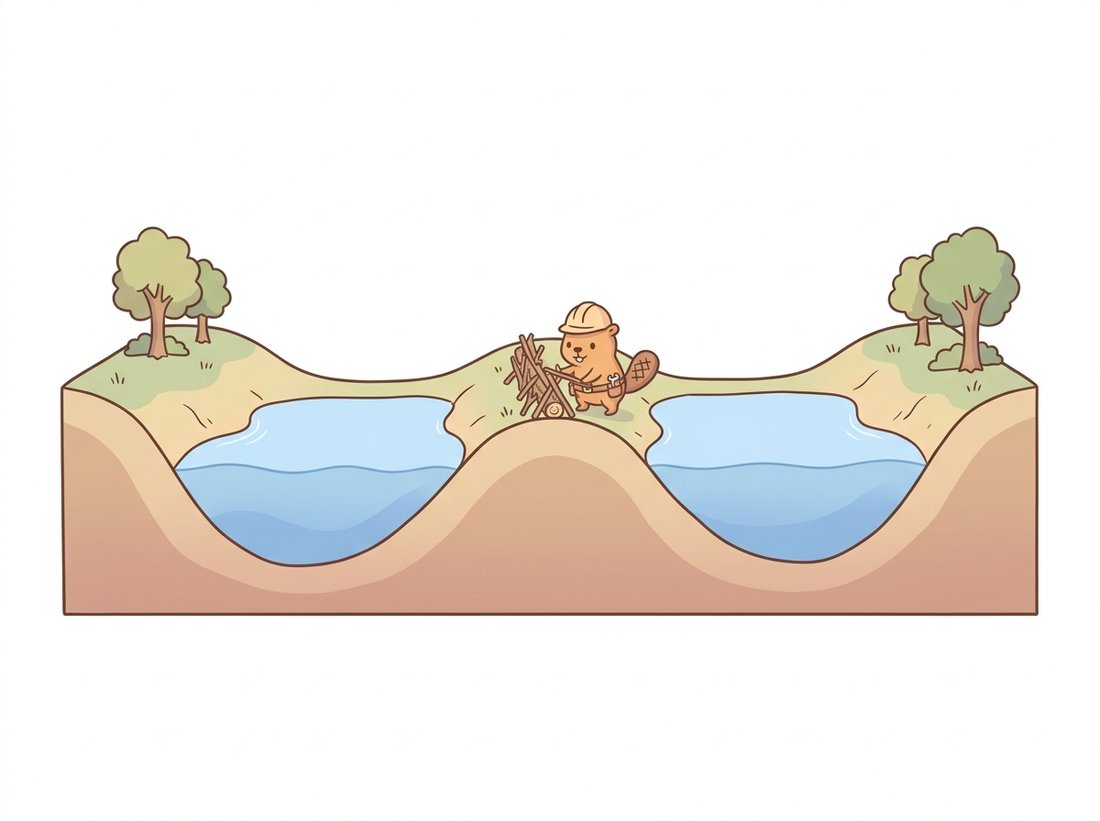
The immersion algorithm of Vincent and Soille (1991) builds these basins by simulating a flood. Imagine piercing a hole at each regional minimum and slowly immersing the whole landscape in water. Water wells up from each minimum, filling its basin. Whenever the water from two distinct basins would meet, a dam is erected at that location to keep them separate. When the entire surface is submerged, the dams that remain are the watershed lines, and the basins they enclose are the segments. Figure 11.3.1 shows this flooding for a one-dimensional intensity profile with two valleys.

Applied naively to a raw image, the surface to flood is usually the gradient magnitude, not the intensity itself, because object boundaries are where the gradient is high (ridges) and object interiors are where it is low (valleys). Flooding the gradient image puts watershed lines on the edges, which is what we want. The gradient comes straight from the Sobel operator of Chapter 3.

2. The Oversegmentation Problem Basic

There is a catch, and it is severe. Real images contain a regional minimum almost everywhere, because sensor noise creates thousands of tiny local dips. Since the immersion algorithm starts a basin at every regional minimum, naive watershed produces one segment per minimum, which means hundreds or thousands of segments where you wanted five. This is the notorious oversegmentation of the watershed, and it is so reliable that an unguided watershed is essentially never used in practice.

3. Marker-Controlled Watershed Intermediate

The fix that makes watershed useful is marker-controlled watershed. Instead of letting every regional minimum seed a basin, you supply a small set of markers, one per object you want, plus one for the background, and force the flood to originate only from those markers. The result has exactly as many segments as you have markers (plus background), and the watershed lines fall on the ridges between marked regions. The genius is in how the markers are obtained for the touching-objects case, and it threads together three tools you already have:

1. Threshold the image to a binary foreground mask (Otsu's method from Chapter 2 is the usual choice).
2. Compute the distance transform of the foreground (from Chapter 6): each foreground pixel is labeled with its distance to the nearest background pixel. The center of each blob is a peak; the thin neck where two blobs touch is a valley.
3. Threshold the distance transform high to get one sure-foreground marker per blob (the peaks survive, the neck does not), label them with connected components, and flood the negated gradient or the negated distance from those markers.

Because the distance-transform peak of each blob is separated by the low ridge at the neck, the markers are distinct, and watershed dams the flood exactly at the neck. This is the standard recipe for separating touching cells, coins, or grains, and Figure 11.3.2 illustrates why the distance transform turns the touching-objects problem into a watershed it can solve.

The OpenCV implementation, cv2.watershed, takes a marker image of 32-bit integer labels: positive integers for known regions, zero for "unknown" pixels to be assigned, and it writes -1 onto the watershed lines. Below is the complete coin-separation pipeline.

import cv2
import numpy as np

img = cv2.imread("coins.jpg")
gray = cv2.cvtColor(img, cv2.COLOR_BGR2GRAY)

# 1. Otsu threshold -> binary foreground (coins white, background black).
_, binary = cv2.threshold(gray, 0, 255, cv2.THRESH_BINARY_INV + cv2.THRESH_OTSU)

# 2. Clean the mask and find SURE background by dilating.
kernel = np.ones((3, 3), np.uint8)
opened = cv2.morphologyEx(binary, cv2.MORPH_OPEN, kernel, iterations=2)
sure_bg = cv2.dilate(opened, kernel, iterations=3)

# 3. Distance transform -> peaks are coin centers. Threshold high for sure FG.
dist = cv2.distanceTransform(opened, cv2.DIST_L2, 5)
_, sure_fg = cv2.threshold(dist, 0.5 * dist.max(), 255, 0)
sure_fg = sure_fg.astype(np.uint8)

# 4. Unknown = background minus foreground; label markers with connected comps.
unknown = cv2.subtract(sure_bg, sure_fg)
n_markers, markers = cv2.connectedComponents(sure_fg)
markers = markers + 1               # so sure background is 1, not 0
markers[unknown == 255] = 0         # mark unknown region with 0

# 5. Flood. cv2.watershed writes -1 on the boundary ridges.
markers = cv2.watershed(img, markers)
img[markers == -1] = [0, 0, 255]    # paint watershed lines red

n_objects = n_markers - 1           # minus the background label
print("coins separated:", n_objects)
# coins separated: 24

The chain of operations is worth pausing on, because every link is a tool from an earlier chapter: thresholding from Chapter 2, morphological opening and dilation and the distance transform from Chapter 6, connected components for marker labeling, and watershed itself to flood. The watershed is the climax, but it is the distance transform that does the conceptual heavy lifting, turning "two blobs that touch" into "two peaks separated by a valley" that the flood can resolve.

import numpy as np
from scipy import ndimage as ndi
from skimage.segmentation import watershed
from skimage.feature import peak_local_max

dist = ndi.distance_transform_edt(binary_mask)            # distance transform
coords = peak_local_max(dist, min_distance=20, labels=binary_mask)
markers = np.zeros(dist.shape, dtype=int)
markers[tuple(coords.T)] = np.arange(1, len(coords) + 1)  # one label per peak
labels = watershed(-dist, markers, mask=binary_mask)      # flood the negated distance
print("objects:", labels.max())

4. Where Watershed Fits, and Where It Hands Off Intermediate

Watershed earns its keep whenever objects are blob-like and the main difficulty is that they touch: cells, coins, grains, pills, bubbles, nuclei. Its weaknesses are equally specific. It struggles with elongated or branching objects whose distance transform has no single clean peak, with objects of wildly varying size (one min_distance cannot fit all), and with scenes where the gradient surface is noisy enough that even smoothing leaves spurious basins. And like every method in this chapter so far, it knows nothing about what an object is; it separates blobs whether or not they are meaningful.

There is one more conceptual gap. Watershed makes a hard, local commitment, the dam goes at the ridge, full stop, with no notion of a global cost that might prefer a slightly different cut. The next section, Section 11.4, replaces local commitment with global optimization: it writes the segmentation as the minimum of an energy over the whole image and solves it exactly for the two-region case. That global view is what finally lets a segmenter trade a little local boundary accuracy for a lot of global coherence, and it is the bridge to the learned segmentation of Chapter 24.