"Tell me which pixels are definitely yours and which are definitely mine. I will find the cheapest possible fence between us, and I promise it will be the globally optimal fence, not merely a locally convenient one."
A Min-Cut Solver Who Refuses to Settle for Greedy
Graph-based segmentation reframes the whole problem as cutting a graph: pixels are nodes, similarities between neighbors are edge weights, and a segmentation is the set of edges you sever to split the graph into pieces. This reframing buys something none of the previous methods had: a single global objective whose exact minimum is the segmentation. For the two-region foreground/background case, the celebrated min-cut/max-flow theorem makes that minimum computable in low-order polynomial time, so graph cuts find the best partition over the entire image rather than the one greedy local steps stumbled into. GrabCut wraps this engine in an interface so friendly it became the one-click background remover in every photo editor: draw a box around the subject, and an iterated graph cut, refined by learned color models, peels the foreground from the background.
The previous three sections each made local decisions: clustering judged each pixel alone, region growing committed greedily one neighbor at a time, watershed dammed at the nearest ridge. None of them optimized anything global, and so none could trade a small local concession for a large global gain. This section changes the frame entirely. We will phrase segmentation as the minimization of an energy that scores an entire labeling of the image at once, balancing how well each pixel's label fits its own appearance against how much neighboring pixels disagree. Remarkably, for two labels this energy can be minimized exactly, which is what gives graph cuts their reputation. The graph machinery here is the same that underlies the robust fitting and consensus ideas of Chapter 10, now applied to dense per-pixel labeling rather than sparse model fitting.
1. Segmentation as Energy Minimization Intermediate
Assign each pixel $p$ a binary label $\ell_p \in \{0, 1\}$ (background or foreground). Score a complete labeling $\ell$ with an energy built from two terms:
$$E(\ell) = \underbrace{\sum_{p} D_p(\ell_p)}_{\text{data (unary) term}} + \lambda \underbrace{\sum_{(p,q) \in \mathcal{N}} V_{pq}(\ell_p, \ell_q)}_{\text{smoothness (pairwise) term}}$$
The data term $D_p(\ell_p)$ is the penalty for giving pixel $p$ the label $\ell_p$ based on $p$'s own appearance: small if $p$'s color matches the foreground model and you label it foreground, large if it does not. The smoothness term $V_{pq}$ penalizes neighboring pixels $p$ and $q$ taking different labels, and it is weighted to be small (cheap to cut) where the image gradient is large, because a label boundary is expected at an edge. The trade-off weight $\lambda$ sets how much the result prefers smooth boundaries over fitting every pixel's appearance. This is exactly the local-evidence-versus-global-consistency tension named in the chapter overview, now written as arithmetic.
The standard smoothness term uses a contrast-sensitive weight,
$$V_{pq}(\ell_p, \ell_q) = [\ell_p \ne \ell_q] \cdot \exp\!\left(-\frac{\lVert I_p - I_q \rVert^2}{2\sigma^2}\right),$$
which is near zero when $p$ and $q$ straddle a strong edge (so cutting there is cheap) and near one when they look alike (so cutting there is expensive). The bracket $[\cdot]$ is 1 when the labels differ and 0 otherwise, so identically labeled neighbors cost nothing.
2. The Min-Cut/Max-Flow Connection Advanced
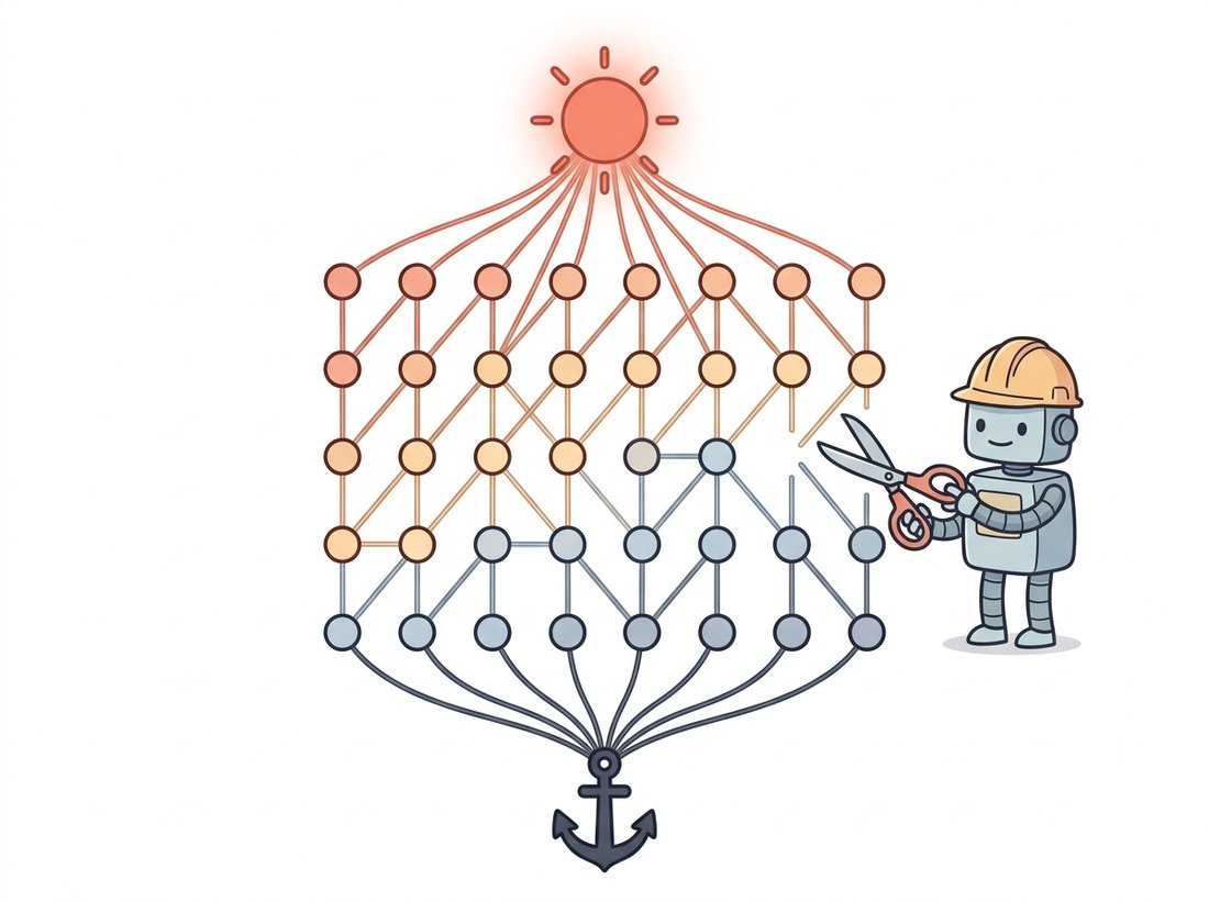
Here is the beautiful part. Build a graph with one node per pixel plus two special terminal nodes, the source $S$ (foreground) and the sink $T$ (background). Connect every pixel to both terminals with edges whose weights encode the data term $D_p$, and connect neighboring pixels with edges whose weights encode the smoothness term $V_{pq}$. An $s$-$t$ cut partitions the nodes into the side still connected to $S$ (labeled foreground) and the side connected to $T$ (labeled background). Each pixel starts wired to both terminals, and a cut must sever exactly one of those two wires per pixel. Sever its $T$-edge and the pixel stays on the $S$ side, so it is labeled foreground; sever its $S$-edge and it becomes background. That is how a single cut hands every pixel a label at once. The cost of the cut is the sum of the weights of the severed edges, which is exactly $E(\ell)$ for the corresponding labeling. The illustration below pictures this wiring as cutting the cheapest fence between source and sink.
So minimizing the energy is the same as finding the minimum-cost $s$-$t$ cut. And the max-flow/min-cut theorem says the minimum cut equals the maximum flow from $S$ to $T$, which efficient algorithms (the Boykov-Kolmogorov solver is the vision standard) compute in low-order polynomial time. For two labels and a submodular smoothness term (one that never rewards two neighbors for disagreeing, which the contrast-sensitive penalty above satisfies), this gives the globally optimal segmentation, not an approximation.
Why exactly two labels? The restriction is not arbitrary: an $s$-$t$ cut places every node on exactly one side, the source side or the sink side, so the construction can encode precisely two labels and no third. With three or more labels there is no single cut whose cost equals the energy, the exact problem becomes NP-hard, and methods like alpha-expansion (Section 5) fall back to a sequence of two-label cuts that find a strong local minimum rather than the guaranteed global one.
Within that two-label case, though, sit with how strong the claim is. A one-megapixel image has $2^{1{,}000{,}000}$ possible foreground/background labelings, an unimaginably vast space, and yet a single max-flow computation returns the one labeling with the lowest energy of them all, exactly, in a fraction of a second. The greedy methods of the previous three sections searched a sliver of that space and hoped; the min cut surveys all of it and proves. Figure 11.4.1 shows the graph construction for a tiny image.
Every earlier method in this chapter could be defeated by an unlucky local decision: a leaked region, a misplaced seed, an over-eager merge. Graph cuts cannot, for the two-label case, because they return the exact global minimum of the energy. If the energy is a good model of what you want, the answer is provably the best one. This is a genuinely different guarantee from "it usually works", and it is why interactive segmentation tools chose graph cuts: a user who corrects a mistake by scribbling a few extra foreground or background pixels is editing the data term, and the next min cut is again globally optimal under the new constraints. The catch, which the next section confronts, is that the energy needs good appearance models to score the data term, and those are not given for free.
The max-flow/min-cut theorem that makes graph cuts globally optimal was not invented for vision. Ford and Fulkerson derived it in 1956 at the RAND Corporation, and a once-classified motivation was estimating how much rail traffic the Soviet network could push toward Eastern Europe, and, by the dual min-cut, which links to bomb to choke it. The same arithmetic that planned to sever a railway now severs the cheapest fence between your foreground and your background. When GrabCut peels a cat off a couch, it is solving a 1950s logistics problem one pixel-grid at a time.
3. GrabCut: Graph Cuts From a Single Box Intermediate
Pure graph cuts need the foreground and background appearance models up front to compute the data term, but a user is not going to hand-label color distributions. GrabCut (Rother et al., 2004) solves this with an iterative bootstrap so light-touch it feels like magic: the user draws a single bounding box around the subject, and everything else follows automatically.
- Initialize. Pixels outside the box are definite background; pixels inside are "probably foreground". Fit a Gaussian Mixture Model (GMM) of colors to each group. A GMM here is simply a flexible color model: it describes a group's colors as a weighted blend of a few Gaussian blobs in color space, so it can capture "the foreground is mostly skin tones plus some dark hair" rather than a single average color.
- Assign. Use the two GMMs to compute the data term $D_p$ for every pixel, then run a graph cut to get a current foreground/background labeling.
- Re-learn. Refit the GMMs to the new labeling, which now describes the colors better than the crude box did.
- Repeat steps 2 and 3 until the labeling stops changing (a few iterations suffice).
Each iteration is a globally optimal graph cut under the current models; alternating cut and model-refit drives the energy down monotonically. The result is a clean foreground mask from a single rectangle of user input. OpenCV exposes the whole loop as cv2.grabCut.
import cv2
import numpy as np

img = cv2.imread("portrait.jpg")
mask = np.zeros(img.shape[:2], np.uint8)        # 0 = sure BG, filled by grabCut
bgd_model = np.zeros((1, 65), np.float64)        # GMM scratch buffers (5 components)
fgd_model = np.zeros((1, 65), np.float64)

# Bounding box (x, y, w, h) loosely around the subject; that is the ONLY input.
rect = (60, 40, 380, 460)
cv2.grabCut(img, mask, rect, bgd_model, fgd_model, iterCount=5,
            mode=cv2.GC_INIT_WITH_RECT)

# grabCut writes 4 codes: 0/2 = background, 1/3 = foreground. Collapse to binary.
fg = np.where((mask == cv2.GC_FGD) | (mask == cv2.GC_PR_FGD), 1, 0).astype(np.uint8)
cutout = img * fg[:, :, None]                    # apply the mask
print("foreground pixels:", int(fg.sum()), "of", fg.size)
# foreground pixels: 96214 of 230000cv2.grabCut. The five iterations alternate a globally optimal graph cut with a Gaussian-mixture color-model refit; the only user input is the bounding rectangle. The returned mask uses four codes that collapse to a binary foreground mask.
When the box alone is not enough, for instance a background object whose color matches the subject, GrabCut accepts user touch-ups: re-run with mode=cv2.GC_INIT_WITH_MASK after the user paints a few pixels as definite foreground (cv2.GC_FGD) or definite background (cv2.GC_BGD). Those strokes become hard constraints on the data term, and the next cut respects them while staying globally optimal everywhere else. This scribble-and-recut interaction is the direct ancestor of the click-and-refine loops in promptable models like SAM, covered in Chapter 24.
4. Felzenszwalb-Huttenlocher: Fast, Unsupervised, No Box Intermediate
Graph cuts and GrabCut both need user input or appearance models. For fully automatic oversegmentation, the Felzenszwalb-Huttenlocher (2004) algorithm is the graph-based workhorse, and it runs in near-linear time. It treats the image as a graph with an edge between each pair of neighboring pixels weighted by their color difference, sorts all edges by weight, and greedily merges the two regions joined by the next edge if that edge is weaker than the internal variation already present in both regions, plus a size-dependent slack controlled by a scale parameter $k$. The adaptive predicate is the clever part: it allows large merges in high-variability (textured) regions while keeping fine boundaries in smooth ones, so a single $k$ behaves sensibly across heterogeneous images.
from skimage.segmentation import felzenszwalb, mark_boundaries
from skimage import data
import numpy as np

img = data.coffee()                              # an RGB photo
# scale: higher -> larger regions; sigma: pre-smoothing; min_size: merge tiny regions.
seg = felzenszwalb(img, scale=300, sigma=0.7, min_size=100)
print("regions:", seg.max() + 1)                 # label image, one int per region
# regions: 64

overlay = mark_boundaries(img, seg) # draw region borders for displayscale parameter trades region count against size; the adaptive boundary predicate is what lets one setting handle both smooth and textured areas of the same photo.Felzenszwalb output is rarely a final segmentation, it oversegments, but it is an excellent initialization: feed its regions into a region adjacency graph (as in Section 11.2) for further merging, or use it as the superpixel substrate of Section 11.5. It is the fast, label-free counterpart to the user-driven graph cuts above.
A correct graph-cut segmenter from scratch means implementing a max-flow solver (Boykov-Kolmogorov is several hundred careful lines), building the n-link and t-link graph, and, for GrabCut, fitting and refitting Gaussian mixture models in a loop. The two library calls above replace all of it:
cv2.grabCut: the full GMM-plus-graph-cut iteration in one call. From-scratch, this is 300-plus lines (max-flow solver, GMM EM, the alternation loop); the library is a single function with five well-chosen arguments.skimage.segmentation.felzenszwalb: the near-linear graph segmentation with its union-find region merging and adaptive predicate, roughly 150 lines of subtle code, as one call.
The libraries also bring the performance that matters: OpenCV's GrabCut uses the optimized Boykov-Kolmogorov max-flow, and scikit-image's Felzenszwalb uses an efficient disjoint-set union-find, both far faster and more numerically careful than a teaching implementation. Reach for these whenever you need the result rather than the lesson.
An online marketplace required every seller to upload product photos on a clean white background, but sellers shot products on kitchen tables, carpets, and car seats. Hiring photo editors did not scale to tens of thousands of daily uploads. The engineering team shipped an automatic background remover built on GrabCut: detect the largest central object with a quick saliency pass to propose the bounding box, run cv2.grabCut for five iterations, and composite the foreground onto white. This handled the large majority of uploads with no human in the loop and no training data.
The decision that made it production-grade was the fallback path. For the roughly twelve percent of images where GrabCut's box-only result was poor (busy backgrounds, products colored like their surroundings), the system surfaced the result to a lightweight web tool where a reviewer painted two or three foreground and background strokes and re-ran GrabCut in GC_INIT_WITH_MASK mode, fixing each in seconds because the recut stayed globally optimal under the new strokes. The lesson: a classical, training-free graph cut cleared most of the volume cheaply, and the interactive scribble path turned the hard tail into a few seconds of human work rather than a full manual edit. Years later the team replaced the core with a learned matting model, but the box-then-scribble interaction they designed around GrabCut carried over unchanged.
You now have every piece needed to build the thing the practical example describes: a folder-in, folder-out background remover with no training data. Loop over a directory of product or portrait photos, propose a bounding box for each (start with a fixed inner rectangle, then upgrade to an automatic box from a saliency or simple center-of-mass heuristic), run cv2.grabCut for five iterations in GC_INIT_WITH_RECT mode, and composite the foreground onto a white or transparent background. Add a "review queue" that flags any image where the foreground mask covers too little or too much of the box, the same hard-tail fallback that made the e-commerce pipeline production-grade, and let a second pass accept a few GC_FGD and GC_BGD scribbles to fix those via GC_INIT_WITH_MASK. The result is an interview-ready demo that turns the globally optimal graph cut of this section into a batch tool, and it doubles as a clean before-and-after for a portfolio. For a stretch, save a four-channel PNG with the GrabCut mask as the alpha channel so the cutouts drop cleanly onto any layout.
5. The Ceiling of Color-Only Energy Intermediate
Graph cuts give the globally optimal segmentation for the energy you wrote down, and that qualifier is the whole limitation. The standard energy scores the data term from color models and the smoothness term from local contrast, so it has no notion of objects, parts, or semantics. A graph cut will happily separate a red shirt from a red wall along the faint shadow between them, or fail to separate a person from a same-colored door, because color and contrast are all it knows. Multi-region extensions (alpha-expansion for more than two labels) and the normalized-cut criterion of Shi and Malik exist, but they do not add semantics; they only refine the same appearance-based objective.
Because graph cuts return the exact global minimum of the energy, it is tempting to read the result as the right segmentation. It is not: it is the best labeling for the energy you wrote down, and that energy knows only color and local contrast. If the foreground and background share a color, the optimal cut will confidently merge them; if a strong shadow crosses one object, the optimal cut may split it. The optimality guarantee is about the solver, not about the world. This is exactly why a worse-looking result from a different method can still be more useful, and why GrabCut needs the user's box and scribbles to inject the information color alone cannot supply. Optimal-for-a-bad-model is still wrong, and no amount of better optimization fixes a data term that cannot see objects.
The energy framework itself, however, is one of the most durable ideas in the chapter, because it survived the transition to deep learning almost intact. When Chapter 24 bolts a Conditional Random Field onto the output of a fully convolutional network, the CRF is this exact energy, with the data term now supplied by the network's per-pixel logits (learned, semantic) and the smoothness term still the contrast-sensitive pairwise penalty of this section. The classical insight, that good segmentation balances local evidence against pairwise consistency, was right; only the source of the local evidence changed. The last section of this chapter, Section 11.5, takes a different exit: rather than improve the energy, it shrinks the problem, replacing millions of pixel nodes with a few hundred superpixel nodes so the graph methods of this section run far faster on a far smaller graph.
The graph-cut energy did not lose to deep learning so much as get absorbed by it. DeepLab (Chen et al., the v1 and v2 lines, with the CRF-as-RNN formulation of Zheng et al., ICCV 2015) appended a dense CRF, the very energy of this section, to a CNN's logits, and the contrast-sensitive pairwise term sharpened blurry network boundaries enough to win benchmarks for years. Modern promptable models took the interactive thread instead: SAM (Kirillov et al., ICCV 2023) and SAM 2 (Ravi et al., ICLR 2025) replace GrabCut's box and scribbles with learned prompt encoders, so a click yields a mask without any per-image GMM or max-flow, but the user-in-the-loop spirit of GrabCut is unmistakable. On the unsupervised side, normalized cuts came back as a deep tool: CutLER (Wang et al., CVPR 2023) runs normalized cuts on self-supervised features to discover object masks with no labels, exactly Shi and Malik's criterion with the affinity matrix now built from learned embeddings. Across all three, the classical structure, an energy or a cut, persists; the weights it operates on became learned.
6. Normalized Cuts: Removing the Small-Cut Bias Advanced
The min-cut of Section 2 has a quiet flaw that the two-terminal foreground/background setup hides. When there is no source and sink to anchor the partition, and we simply ask for the cheapest cut that splits the graph into two parts $A$ and $B$, the cost
is the sum of the affinity weights $w(u,v)$ on every edge crossing the partition. Minimizing this raw cut is biased toward slicing off a tiny, isolated group of nodes: a single node weakly connected to the rest is cut by severing just its few thin edges, and that is almost always cheaper than splitting the graph into two substantial halves. The cut criterion rewards small partitions for the wrong reason, namely that a small set simply has fewer edges to cut, not that it is a more natural grouping. This is precisely why min-cut, so well behaved with terminals, misbehaves as a generic clustering objective.
Shi and Malik (2000) fix the bias by normalizing the cut against the total connection each part has to the whole graph. Define the association of a set $A$ with all vertices $V$ as
the total weight from $A$ to every vertex (itself included). The normalized cut of a partition $(A, B)$ is then
Read each term as the fraction of $A$'s total connectivity that is spent on the cut, plus the same fraction for $B$. A tiny group $A$ now pays dearly: its association $\operatorname{assoc}(A, V)$ is small, so even a small numerator makes the first ratio large, and the criterion stops preferring to peel off singletons. The minimum of $\operatorname{Ncut}$ falls where both parts are substantial and the edges between them are genuinely weak, which is the balanced partition we wanted all along. The same normalization, written as $\operatorname{Nassoc}(A,B) = \operatorname{assoc}(A,A)/\operatorname{assoc}(A,V) + \operatorname{assoc}(B,B)/\operatorname{assoc}(B,V)$, measures within-group tightness, and one can show $\operatorname{Ncut}(A,B) = 2 - \operatorname{Nassoc}(A,B)$, so minimizing the cut between groups is identical to maximizing the association within them.
The min-cut asks an absolute question, "how much edge weight must I sever?", and a small isolated group always answers it cheaply, because a small group simply has few edges to begin with. Normalized cuts asks a relative question, "what fraction of each group's own connectivity does this cut destroy?", and a small group can no longer hide behind its small edge count: severing a singleton destroys nearly all of that singleton's connectivity, so the ratio is near its maximum, not its minimum. Dividing by the association is exactly the operation that converts "few edges" from a reward into a neutral fact, which is why a criterion built from the very same cut weights produces balanced segments instead of slivers.
Minimizing $\operatorname{Ncut}$ over all partitions is NP-hard, but Shi and Malik show it admits a clean continuous relaxation. Collect the affinities into the symmetric weight matrix $W$ with $W_{ij} = w(i,j)$, and form the diagonal degree matrix $D$ with $D_{ii} = \sum_j W_{ij}$, the total weight incident on node $i$. Encode the partition by an indicator vector $x \in \{1, -b\}^n$ (positive on $A$, a fixed negative constant on $B$). Substituting this indicator into $\operatorname{Ncut}$ and rearranging turns the combinatorial objective into a Rayleigh quotient in a real-valued vector $y$, and minimizing that quotient is exactly the generalized eigenvalue problem
The matrix $L = D - W$ is the graph Laplacian. Its smallest eigenvalue is $\lambda_0 = 0$ with the trivial eigenvector $y_0 = \mathbf{1}$ (the all-ones vector), which assigns every node to the same side and so encodes no cut at all. The informative solution is the eigenvector of the second-smallest eigenvalue, the Fiedler vector: its real-valued entries give a soft assignment of nodes to the two parts, and thresholding them (at zero, the median, or the split that yields the lowest $\operatorname{Ncut}$) produces the discrete segmentation. Subsequent eigenvectors, those of the third- and fourth-smallest eigenvalues, carry progressively finer partitioning information and can be used to subdivide the image into more than two regions.
This construction is the prototype of spectral clustering: represent data as an affinity graph, build its Laplacian, and read the cluster structure off the lowest nontrivial eigenvectors. Normalized cuts is the segmentation-flavored instance of that general recipe, and the same affinity-plus-Laplacian machinery reappears whenever a grouping problem is posed as a balanced graph partition, including the learned-affinity revival noted in the research-frontier callout above.
Let $W$ be the symmetric affinity matrix and $D$ the diagonal degree matrix with $D_{ii} = \sum_j W_{ij}$. (a) Show that $y = \mathbf{1}$ (the all-ones vector) satisfies $(D - W)\,y = 0$, so it is an eigenvector of the generalized problem $(D - W)y = \lambda D y$ with eigenvalue $\lambda = 0$, and explain why this trivial solution corresponds to "cut nothing" and must therefore be discarded. (b) Using the partition indicator $x_i = 1$ for $i \in A$ and $x_i = -1$ for $i \in B$, verify that $\operatorname{cut}(A,B) = \tfrac{1}{4}\sum_{i,j} W_{ij}(x_i - x_j)^2 = \tfrac{1}{4}\, x^\top (D - W)\, x$, which is the numerator that the Laplacian quadratic form measures. (c) Argue from these two facts that minimizing the normalized cut relaxes to minimizing the Rayleigh quotient $y^\top (D - W) y / (y^\top D y)$ subject to $y^\top D \mathbf{1} = 0$ (orthogonality to the trivial solution), whose minimizer is the Fiedler vector, the eigenvector of the second-smallest eigenvalue.
Consider the energy $E(\ell) = \sum_p D_p(\ell_p) + \lambda \sum_{(p,q)} V_{pq}(\ell_p, \ell_q)$. Describe qualitatively what the optimal segmentation looks like in three regimes: (a) $\lambda = 0$, (b) $\lambda \to \infty$, and (c) a moderate $\lambda$. For each, explain whether the result is dominated by the data term, the smoothness term, or a balance, and relate $\lambda = 0$ back to the speckle problem of Section 11.1's clustering.
Run cv2.grabCut on a photo with a single bounding box and display the result. Then identify a region it got wrong, programmatically paint a small patch of that region as cv2.GC_FGD or cv2.GC_BGD in the mask, and re-run with mode=cv2.GC_INIT_WITH_MASK. Show before and after, and report how many foreground pixels changed. Explain in terms of hard constraints on the data term why the second cut still respects your strokes while improving the rest of the boundary.
Run skimage.segmentation.felzenszwalb on one image across a range of scale values while holding sigma and min_size fixed. Plot region count versus scale and, for three representative scales, overlay the region boundaries on the image. Identify a textured region and a smooth region in the photo, and explain how the adaptive boundary predicate produces large regions in the textured area and small ones in the smooth area at the same scale setting. Contrast this adaptivity with the single global threshold of region growing in Section 11.2.
Introduces the normalized-cut criterion that removes min-cut's bias toward small isolated groups by dividing the cut cost by each part's total association, and shows that minimizing it relaxes to the generalized eigenproblem $(D - W)y = \lambda D y$ solved by the second-smallest (Fiedler) eigenvector. The founding paper of spectral segmentation, and the criterion CutLER revives on self-supervised features.