Segmentation as Clustering: K-Means & Mean-Shift

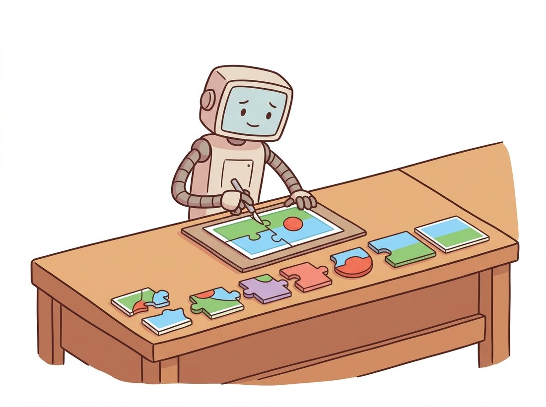
"I sorted your pixels into five tidy groups. You wanted a cat, a sofa, and some sky? I gave you five shades of beige. We clearly value different things."

A Color-Quantizing K-Means Instance With Strong Opinions About k

In the previous chapter we hunted for sparse keypoints, the rare pixels distinctive enough to match across views. This section inverts the goal. We want a label for every pixel, and we want pixels that look alike to share a label. The cleanest framing of that wish is clustering: define a feature vector for each pixel, drop all of those vectors into a space, and group the ones that fall close together. Segmentation then becomes a side effect of clustering, the cluster index assigned back to the pixel's location is its segment. This view connects directly to the histograms and thresholds of Chapter 2: a threshold is a one-dimensional, two-cluster special case of exactly this idea.

1. Pixels as Points in a Feature Space Basic

A grayscale image of $H \times W$ pixels can be unrolled into $HW$ points on the intensity line $[0, 255]$. A color image becomes $HW$ points in a three-dimensional color cube. The choice of which features to use is the single most consequential decision in clustering-based segmentation, more consequential than the clustering algorithm itself. Three common choices, in increasing richness:

• Color only, a 3-vector $(R, G, B)$ or, better, $(L, a, b)$ in a perceptually uniform space. Pixels are grouped purely by appearance; two regions of identical color anywhere in the image merge.
• Color plus position, a 5-vector $(L, a, b, x, y)$. Adding the spatial coordinates, scaled by a weight, biases the clustering toward compact, spatially coherent blobs. This is the feature that makes superpixels work in Section 11.5.
• Color plus texture, where each pixel carries a vector of filter-bank responses (Gabor energies, the local binary patterns hinted at in Chapter 9). This separates regions that share a mean color but differ in pattern, like grass from a green wall.

Why prefer CIELAB over raw RGB? Because clustering measures distance, and in RGB the Euclidean distance between two colors does not match how different they look to a human eye. CIELAB was designed so that equal Euclidean steps correspond to roughly equal perceived color changes, which means a K-Means boundary drawn at constant distance in Lab lands where a person would also draw it. Converting is one OpenCV call, and it routinely improves the segmentation for free. Figure 11.1.1 shows the same image as a cloud of points in feature space, the geometry that every clustering method below operates on.

2. K-Means: Partition Into k Groups Basic

K-Means is the workhorse. Given $n$ points and a target count $k$, it seeks $k$ centers (centroids) $\mu_1, \dots, \mu_k$ that minimize the total squared distance from each point to its nearest center:

$$J = \sum_{i=1}^{n} \min_{j \in \{1,\dots,k\}} \lVert x_i - \mu_j \rVert^2$$

This objective is non-convex, so K-Means does not solve it exactly. Instead it runs Lloyd's algorithm, an alternation that is guaranteed to decrease $J$ at every step until it stops moving:

1. Assign: give each point to its nearest centroid.
2. Update: move each centroid to the mean of the points assigned to it.
3. Repeat until assignments stop changing.

The catch is that Lloyd's algorithm converges to a local minimum that depends on where the centroids start. Poor initialization gives poor segmentations. The standard fix is k-means++, which seeds centers spread out across the data rather than at random; OpenCV and scikit-learn both default to it. Here is K-Means color segmentation written against OpenCV's cv2.kmeans, which expects the feature matrix as float32.

import cv2
import numpy as np

img = cv2.imread("scene.jpg")                       # uint8 BGR, shape (H, W, 3)
lab = cv2.cvtColor(img, cv2.COLOR_BGR2LAB)          # perceptually uniform space

# Reshape (H, W, 3) -> (H*W, 3) and cast to float32 as cv2.kmeans requires.
features = lab.reshape(-1, 3).astype(np.float32)

K = 5
criteria = (cv2.TERM_CRITERIA_EPS + cv2.TERM_CRITERIA_MAX_ITER, 100, 0.2)
# attempts=10: run Lloyd 10 times from different seeds, keep the lowest-energy run.
compactness, labels, centers = cv2.kmeans(
    features, K, None, criteria, attempts=10, flags=cv2.KMEANS_PP_CENTERS)

centers = centers.astype(np.uint8)                  # one mean color per cluster
quantized = centers[labels.flatten()]               # recolor each pixel by its center
segmented = quantized.reshape(lab.shape)
segmented = cv2.cvtColor(segmented, cv2.COLOR_LAB2BGR)

print("compactness (total within-cluster SSD):", round(compactness, 1))
print("cluster centers (Lab):\n", centers)
# compactness (total within-cluster SSD): 18342105.0
# cluster centers (Lab):
#  [[201  126  142] [ 78 121 131] [148 118 168] [122 130 110] [ 49 128 128]]

The output is a clean partition into five color regions. But notice what it cannot tell you: it found five colors, not five objects. If the cat and the sofa share a beige, they merge; if the sky shades from pale to deep blue, it may split. And because each pixel was clustered in isolation, single stray pixels of an off-color get their own label scattered across the image. K-Means also demands that you commit to $k$ before you look. Choosing it badly is the most common failure, which the next callout addresses.

3. Choosing k: The Elbow and the Silhouette Intermediate

K-Means cannot pick $k$ for you, but two diagnostics narrow the choice. The elbow method plots the objective $J$ (within-cluster sum of squares) against $k$. Adding clusters always lowers $J$, but the curve bends sharply at the "natural" number of clusters and flattens afterward; you pick $k$ at the bend. The silhouette score is more principled: for each point it compares the mean distance to its own cluster against the mean distance to the nearest other cluster, giving a value in $[-1, 1]$, and you pick the $k$ that maximizes the average.

from sklearn.cluster import KMeans
from sklearn.metrics import silhouette_score
import numpy as np

# Subsample 5000 pixels: silhouette on a full image is O(n^2) and far too slow.
rng = np.random.default_rng(0)
sample = features[rng.choice(len(features), 5000, replace=False)]

for k in range(2, 8):
    km = KMeans(n_clusters=k, n_init=10, random_state=0).fit(sample)
    sil = silhouette_score(sample, km.labels_)
    print(f"k={k}  inertia={km.inertia_:11.0f}  silhouette={sil:.3f}")
# k=2  inertia=  742103104  silhouette=0.512
# k=3  inertia=  391204480  silhouette=0.547   <- best silhouette
# k=4  inertia=  268339712  silhouette=0.498
# k=5  inertia=  201118368  silhouette=0.441
# k=6  inertia=  168442096  silhouette=0.402
# k=7  inertia=  148209760  silhouette=0.388

Both diagnostics agree on three clusters for this scene, which is reassuring but not a guarantee. In a cluttered natural image neither metric gives a clean answer, because "the right number of regions" is genuinely ambiguous. That ambiguity is the strongest argument for the next method, which refuses to be told $k$ at all.

4. Mean-Shift: Let the Density Decide Intermediate

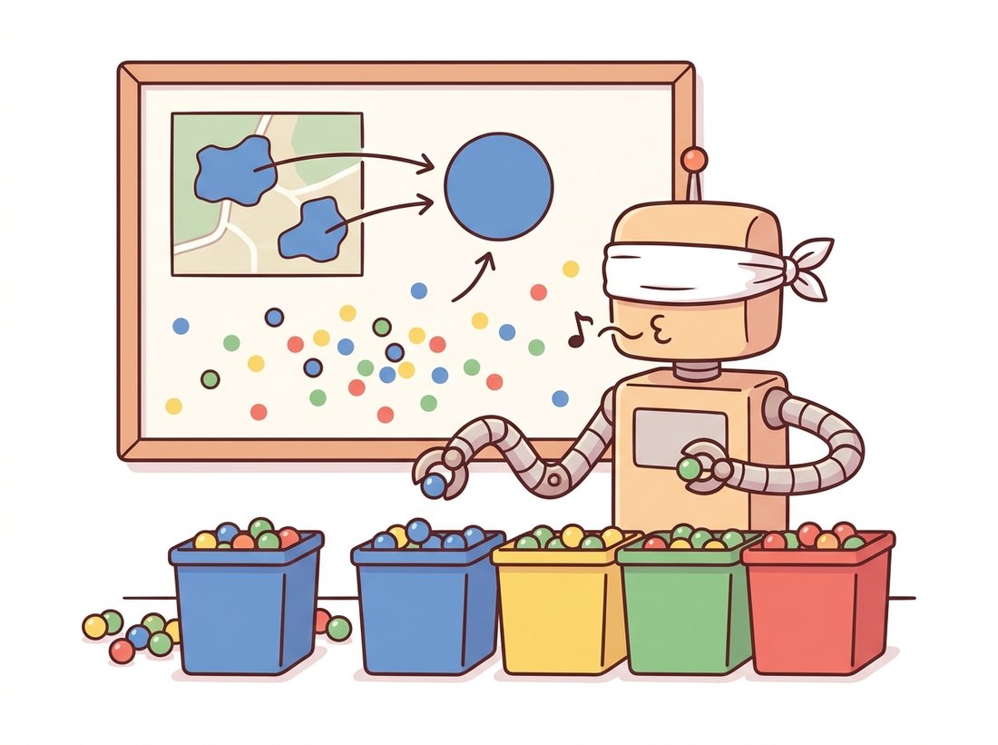
Mean-Shift abandons the idea of a fixed cluster count. It views the feature points as samples from an underlying probability density and seeks that density's modes, its local peaks. Every point climbs uphill toward the nearest peak, and points that arrive at the same peak form one cluster. The number of clusters is whatever number of peaks the data happens to have, given one parameter: the bandwidth $h$, the radius of the window that defines "local".

The climb is elegant. From a point $x$, compute the mean of all points within radius $h$, weighted by a kernel, then shift $x$ to that mean. Repeat. The shift vector,

$$m(x) = \frac{\sum_{i} x_i \, g\!\left(\lVert \frac{x - x_i}{h} \rVert^2\right)}{\sum_{i} g\!\left(\lVert \frac{x - x_i}{h} \rVert^2\right)} - x,$$

always points up the density gradient, so iterating it provably converges to a mode. Figure 11.1.2 traces three points shifting toward the two peaks of a 1D density. A small bandwidth finds many narrow modes (oversegmentation); a large bandwidth merges everything into a few broad modes (undersegmentation). Unlike $k$ in K-Means, bandwidth has a physical meaning, a color-distance scale, which makes it easier to set by intuition.

OpenCV ships a specialized image version, cv2.pyrMeanShiftFiltering, that runs Mean-Shift jointly over color (the range parameter sr) and position (the spatial parameter sp), which is precisely the color-plus-position feature of Section 1. It produces a posterized, edge-preserving image; a connected-components pass then turns the flattened colors into labeled regions.

import cv2
import numpy as np

img = cv2.imread("scene.jpg")
# sp = spatial window radius (pixels), sr = color window radius (Lab/BGR units).
# Larger sr merges more colors; larger sp merges over larger spatial extents.
shifted = cv2.pyrMeanShiftFiltering(img, sp=21, sr=40, maxLevel=1)

# After Mean-Shift the image is piecewise-flat; label the flat regions.
gray = cv2.cvtColor(shifted, cv2.COLOR_BGR2GRAY)
n_labels, labels = cv2.connectedComponents(
    (cv2.Canny(gray, 1, 1) == 0).astype(np.uint8))   # regions = areas with no internal edge
print("Mean-Shift produced", n_labels, "connected regions (no k specified)")
# Mean-Shift produced 37 connected regions (no k specified)

Mean-Shift's gift, automatic cluster count, comes at a cost: it is far slower than K-Means, roughly quadratic in the number of points in a naive implementation, which is why the OpenCV version operates on an image pyramid and why you subsample for the scikit-learn MeanShift estimator. That same mode-seeking iteration reappears as a tracker in Chapter 15, where the "density" is a color histogram and the mode being chased is a moving object.

from sklearn.cluster import KMeans, MeanShift, estimate_bandwidth

# K-Means: parallelized, k-means++ by default, 10 restarts.
km = KMeans(n_clusters=5, n_init=10).fit(features)

# Mean-Shift: bandwidth auto-estimated from a quantile of pairwise distances.
bw = estimate_bandwidth(sample, quantile=0.1, n_samples=500)
ms = MeanShift(bandwidth=bw, bin_seeding=True).fit(sample)
print("Mean-Shift found", len(set(ms.labels_)), "clusters automatically")

5. Why Clustering Is Not Enough Intermediate

Step back and the limitation is structural, not a tuning problem. Clustering segments the feature space, but a segmentation lives in the image grid, and the map between them is lossy in exactly the wrong direction. Two failures follow inevitably:

• Speckle and fragmentation. Because labels are assigned per pixel with no smoothness term, sensor noise scatters single off-color pixels into the wrong cluster, leaving a label image peppered with one-pixel islands. A morphological opening from Chapter 6 cleans the worst of it, but that is a patch, not a cure.
• Merged distinct objects. Two physically separate objects of the same color receive the same label and become one region, because the feature space cannot represent "these are far apart on the grid." No threshold on color distance can separate them.

Both failures trace to the same root: clustering threw away spatial connectivity in Section 1 and never got it back. The remaining sections of this chapter are progressively richer ways to restore it. Section 11.2 grows regions that are connected by construction. Section 11.3 floods a surface so that basins respect topography. Section 11.4 writes spatial smoothness directly into an energy function. Keep the speckle of pure K-Means in mind as the baseline each method improves on.