Dense Flow: Horn-Schunck to Variational Methods

"I had no gradient, no texture, no information of any kind, and yet I have been assigned a velocity. My neighbors voted. Apparently this is called regularization."

A Peer-Pressured Pixel in a Flat Region

Section 15.2 computed excellent flow at corners and refused to answer anywhere else. Many applications cannot accept the refusal. Motion segmentation needs to know which pixels move together; frame interpolation must synthesize every in-between pixel; video compression, action recognition, and the temporally consistent generation of Chapter 36 all want motion everywhere. Dense flow is the answer, and the aperture problem guarantees it cannot come from data alone: most pixels are flat or edge-like, so most of any dense field is necessarily inference. The question is how to infer with discipline.

1. The Horn-Schunck Energy Intermediate

Horn and Schunck's move was to stop solving pixels independently and instead score entire candidate flow fields $(u(x,y), v(x,y))$ with a global energy:

$$ E(u, v) \;=\; \iint \underbrace{\left( I_x u + I_y v + I_t \right)^2}_{\text{data term}} \;+\; \alpha^2 \underbrace{\left( \lVert \nabla u \rVert^2 + \lVert \nabla v \rVert^2 \right)}_{\text{smoothness term}} \; dx\, dy . $$

The data term is the squared OFCE residual from Section 15.1: it punishes flow that disagrees with observed brightness change. The smoothness term punishes flow fields that vary rapidly, encoding the prior that nearby pixels usually belong to the same surface and move alike. The weight $\alpha$ arbitrates: small $\alpha$ trusts data and yields noisy, gappy flow; large $\alpha$ trusts the prior and yields smooth, blurry flow. If this structure feels familiar, it should: it is the same data-plus-regularizer template as the restoration energies of Chapter 7, with flow in place of the clean image.

Minimizing $E$ with the calculus of variations gives a pair of Euler-Lagrange equations, and discretizing them produces a wonderfully simple update. Writing $\bar{u}$ for the average of $u$ over a pixel's four neighbors (a discrete Laplacian rearranged, as in Chapter 3):

$$ u^{(k+1)} = \bar{u}^{(k)} - I_x \frac{I_x \bar{u}^{(k)} + I_y \bar{v}^{(k)} + I_t}{\alpha^2 + I_x^2 + I_y^2}, \qquad v^{(k+1)} = \bar{v}^{(k)} - I_y \frac{I_x \bar{u}^{(k)} + I_y \bar{v}^{(k)} + I_t}{\alpha^2 + I_x^2 + I_y^2}. $$

Read the update as a negotiation. Start from the neighborhood consensus $(\bar u, \bar v)$, then correct it just enough toward the local constraint line, with the correction scaled by how much gradient evidence the pixel actually has. Where gradients are strong, data wins; where the image is flat ($I_x = I_y = 0$), the update reduces to $u \leftarrow \bar u$: pure neighborhood averaging, which is exactly the heat-equation smoothing of Chapter 4. Information diffuses from textured regions into flat ones, iteration by iteration. Figure 15.3.1 visualizes this filling-in, the defining behavior of every global method.

2. Horn-Schunck From Scratch Intermediate

The update equations translate into remarkably little NumPy. The implementation below follows the original paper's derivative stencils and runs a fixed number of Jacobi-style sweeps; on a 640x480 pair it converges visually in a few hundred iterations and a couple of seconds.

import cv2
import numpy as np

def horn_schunck(im1, im2, alpha=15.0, n_iters=300):
    """Dense flow via Horn-Schunck (1981). Returns (u, v) in px/frame."""
    im1 = im1.astype(np.float32) / 255.0
    im2 = im2.astype(np.float32) / 255.0
    # Derivatives averaged across both frames (the paper's 2x2x2 stencils)
    kx = np.array([[-1, 1], [-1, 1]], np.float32) * 0.25
    ky = np.array([[-1, -1], [1, 1]], np.float32) * 0.25
    kt = np.full((2, 2), 0.25, np.float32)
    Ix = cv2.filter2D(im1, -1, kx) + cv2.filter2D(im2, -1, kx)
    Iy = cv2.filter2D(im1, -1, ky) + cv2.filter2D(im2, -1, ky)
    It = cv2.filter2D(im2, -1, kt) - cv2.filter2D(im1, -1, kt)

    u = np.zeros_like(im1)
    v = np.zeros_like(im1)
    avg = np.array([[0, 1, 0], [1, 0, 1], [0, 1, 0]], np.float32) / 4.0
    denom = alpha**2 + Ix**2 + Iy**2
    for _ in range(n_iters):
        u_bar = cv2.filter2D(u, -1, avg)          # neighborhood consensus
        v_bar = cv2.filter2D(v, -1, avg)
        t = (Ix * u_bar + Iy * v_bar + It) / denom
        u = u_bar - Ix * t                        # consensus, corrected by data
        v = v_bar - Iy * t
    return u, v

u, v = horn_schunck(f0, f1, alpha=15.0)
print(f"mean speed: {np.hypot(u, v).mean():.2f} px/frame")
# Expected on a walking-pedestrian clip: mean speed: 0.83 px/frame

Dense flow needs a dense visualization, and the field settled on one convention: hue encodes direction, saturation or value encodes speed, using the HSV color space from Chapter 1. Once you internalize the color wheel (rightward motion red-ish, downward green-ish, and so on, depending on the wheel's rotation), you can read a flow field at a glance, which is how every flow paper presents results.

def flow_to_color(u, v):
    """Standard HSV flow rendering: hue = direction, value = speed."""
    mag, ang = cv2.cartToPolar(u, v, angleInDegrees=True)
    hsv = np.zeros((*u.shape, 3), np.uint8)
    hsv[..., 0] = (ang / 2).astype(np.uint8)            # OpenCV hue is 0..180
    hsv[..., 1] = 255
    hsv[..., 2] = cv2.normalize(mag, None, 0, 255,
                                cv2.NORM_MINMAX).astype(np.uint8)
    return cv2.cvtColor(hsv, cv2.COLOR_HSV2BGR)

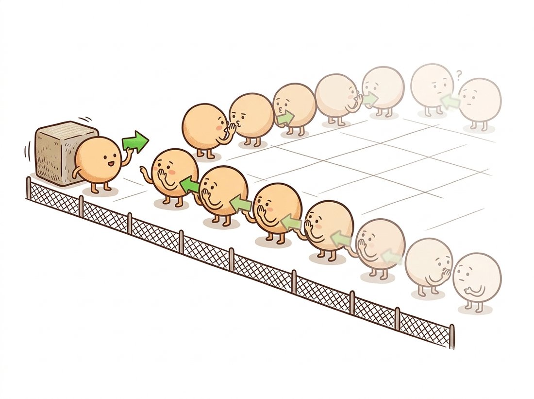
cv2.imwrite("flow_hs.png", flow_to_color(u, v))

3. Beyond Quadratic: Robust and Total-Variation Flow Advanced

Horn-Schunck's two quadratic penalties are also its two weaknesses, and both fail at the same place: boundaries. The quadratic data term squares outliers, so occluded pixels (which satisfy no displacement) dominate the energy. The quadratic smoothness term charges a fortune for sharp changes in flow, so the estimate smears across object boundaries where the true field genuinely jumps; Figure 15.3.1's filling-in, so helpful inside an object, becomes leakage between objects. Notice the rhyme with Chapter 7: quadratic regularization blurred image edges there, and total variation preserved them. The identical medicine works here. Replace squares with gentler penalties, the $L_1$ norm or its smooth Charbonnier approximation $\sqrt{x^2 + \epsilon^2}$, and you get the TV-L1 flow family: data outliers are tolerated rather than catastrophic, and the flow field is encouraged to be piecewise smooth with crisp motion boundaries instead of globally mushy.

The second classical upgrade handles large motion. The linearized data term still only sees sub-pixel displacement, so robust methods embed the energy in the coarse-to-fine warping scheme that Section 15.2 introduced for points: solve on a coarse pyramid level, upsample the flow, warp the second image by it, solve for the residual flow, descend. By the mid-2000s the recipe (robust penalties, graduated warping, sometimes gradient-constancy data terms) defined state-of-the-art flow, and it held the benchmark lead until deep networks arrived.

4. The Practical Workhorses: Farneback and DIS Beginner

When you need dense flow in production OpenCV today, two non-deep options carry almost all the traffic. Farneback (2003) approximates each pixel's neighborhood with a quadratic polynomial and derives displacement from how the polynomial coefficients shift between frames; it is the default cv2.calcOpticalFlowFarneback and a reasonable all-rounder. DIS (Dense Inverse Search, 2016) is the speed champion: it computes fast inverse-compositional Lucas-Kanade matches on a grid of patches, densifies them, and runs a single variational refinement sweep, hitting hundreds of frames per second at usable quality. DIS at its fastest preset powers real-time stabilization and gesture systems on CPUs.

import cv2

prev = cv2.imread("frame_000.png", cv2.IMREAD_GRAYSCALE)
curr = cv2.imread("frame_001.png", cv2.IMREAD_GRAYSCALE)

# Option 1: Farneback, the long-standing default
flow_fb = cv2.calcOpticalFlowFarneback(prev, curr, None, pyr_scale=0.5,
                                       levels=3, winsize=15, iterations=3,
                                       poly_n=5, poly_sigma=1.2, flags=0)

# Option 2: DIS, much faster at comparable quality
dis = cv2.DISOpticalFlow_create(cv2.DISOPTICAL_FLOW_PRESET_MEDIUM)
flow_dis = dis.calc(prev, curr, None)

print(flow_fb.shape, flow_dis.shape)   # (H, W, 2) (H, W, 2): u and v per pixel

5. Evaluating Flow: EPE and the Benchmarks Intermediate

Flow quality is measured by endpoint error (EPE): the Euclidean distance $\sqrt{(u - u^*)^2 + (v - v^*)^2}$ between estimated and ground-truth vectors, averaged over pixels. Ground truth is the hard part; you cannot annotate a million per-pixel vectors by hand. The field's answer was synthetic and instrumented data: MPI-Sintel renders an animated film with exact ground-truth flow (including a notoriously difficult "final" pass with motion blur and fog), and KITTI derives sparse ground truth for driving scenes from LiDAR and egomotion. Treat the numbers with respect and suspicion at once: EPE averages can hide boundary failures, which is why benchmarks also report outlier percentages and why visual inspection of the HSV rendering remains standard practice even in 2026 papers.