Capture-to-Render Pipelines in Practice

"The paper showed a flawless rotating chair. My first capture showed a flawless rotating chair wrapped in glowing fog, sitting in a room that bent like a funhouse mirror. The difference, it turned out, was eleven photos taken while walking backward and one very shiny window."

A Pipeline That Has Met the Gap Between the Demo and the Driveway

Here is the uncomfortable truth the papers never print: the same NeRF or splatting code that produced a flawless rotating chair in Section 27.4 and Section 27.5 will, on your first real capture, just as faithfully produce a chair wrapped in glowing fog inside a room that bends like a funhouse mirror. The method did not change; your inputs did. Both techniques quietly assumed the same thing: a set of images with accurately known camera poses, and that single assumption is where most real projects silently succeed or fail. This closing section is deliberately practical. It treats NeRF and splatting not as models in isolation but as one stage of a pipeline, and it spends its time on exactly the parts that the research papers, optimizing for a clean result on a curated dataset, leave out, which are precisely the parts that decide whether your reconstruction ships or embarrasses you.

1. The Five Stages Beginner

Every capture-to-render project, whatever the final representation, flows through the same five stages, shown in Figure 27.6.1. Capture: shoot photos or video of the scene from many viewpoints. Pose recovery: run structure from motion (COLMAP) to estimate each image's camera pose and a sparse point cloud, the geometry of Chapter 14. Train: fit a NeRF or Gaussian splat to the posed images. Clean: remove floaters and background artifacts, crop to the region of interest. Export: render a video, extract a mesh, or ship the splat to a viewer or engine. The arrows run one way, and an error introduced at any stage propagates to all the stages after it, which is why verification is built into the workflow rather than left to the end.

2. Capturing Well: The Decisions That Matter Most Beginner

More reconstructions are saved or ruined at capture time than anywhere else, because no amount of training fixes missing or contradictory information. The rules are few and they follow directly from how structure from motion and view synthesis work. Overlap: consecutive images must share substantial content (roughly 70 percent) so COLMAP can match features across them, exactly the feature-matching requirement from Chapter 10. Coverage: orbit the subject and vary height, so every surface is seen from several angles; a surface seen once cannot be reconstructed in 3D. Sharpness: avoid motion blur (it poisons feature matching and bakes blur into the field), so move slowly or shoot stills. Constant exposure and focus: lock them, because auto-exposure changes a surface's apparent color between frames and confuses the photometric loss. Avoid the hard cases: textureless walls give COLMAP nothing to match, and reflective or transparent surfaces violate the view-synthesis assumption that a surface point has a consistent (if view-dependent) appearance.

Fun Note: Floaters Are an Honest Answer to a Dishonest Question

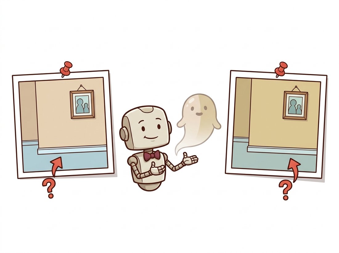
When two of your photos insist a surface is both beige and slightly-more-beige, the optimizer does not throw a tantrum or pick a side. It politely conjures a faint, semi-transparent ghost hanging in mid-air that, viewed from photo one, looks beige, and from photo two, looks slightly-more-beige. The floater is not the model failing; it is the model succeeding at an impossible request with the calm of a bureaucrat who has found a loophole. Blame the brief, not the contractor: fix the captures. The illustration below shows the optimizer politely conjuring its ghost.

3. Pose Recovery and the Verification Habit Intermediate

Stage two runs COLMAP to recover poses, and stage three cannot be trusted unless stage two is verified. The single most valuable habit in this entire pipeline is to look at the sparse reconstruction before training anything. COLMAP reports how many images it successfully registered and produces a sparse point cloud with the camera frustums; a healthy result registers nearly all images and shows a recognizable, undistorted sparse structure. The code below runs the pose-recovery stage through Nerfstudio (which wraps COLMAP) and then inspects the result, the check the museum team of Section 27.4 learned to do the hard way.

# Pose-recovery health gate: read how many images COLMAP actually posed and
# refuse to spend GPU hours on training if too few registered, the cheap check
# that catches poor overlap, motion blur, or reflective surfaces up front.
import json, pathlib

# After running: ns-process-data images --data ./photos --output-dir ./capture
# Nerfstudio writes a transforms.json with one entry per successfully posed image.
transforms = json.loads(pathlib.Path("./capture/transforms.json").read_text())
n_posed = len(transforms["frames"])
print(f"Camera model: {transforms.get('camera_model')}")
print(f"Images successfully posed: {n_posed}")

# A simple health check before committing GPU hours to training.
import glob
n_input = len(glob.glob("./photos/*.jpg"))
ratio = n_posed / max(n_input, 1)
print(f"Registration ratio: {ratio:.0%}")
assert ratio > 0.8, "Too many images failed to register; re-shoot or check overlap/blur."

If registration is poor, the fix is almost always at stages one and two: add images to bridge the gaps where matching failed, mask out reflective regions, or re-shoot the textureless areas with more angle variation. Training a NeRF or splat on bad poses produces the bent-room, double-image artifacts that look like a model problem but are a geometry problem.

4. Training, Cleaning, and Export Intermediate

With verified poses, stages three through five are largely the library-driven commands you saw in the previous two sections: ns-train nerfacto or ns-train splatfacto to fit the field, the live viewer to watch convergence, and ns-export to produce the deliverable. The judgment that remains is in cleaning. Almost every real capture produces some floaters (the inconsistent-data artifacts of subsection 2) and unwanted background. Nerfstudio's viewer lets you set a crop box to keep only the region of interest, which alone removes most distant floaters. For splats, you can additionally prune low-opacity Gaussians and those far from the scene center. The export choice depends on the use: a rendered camera-path video for a presentation, a mesh (via Poisson reconstruction for NeRF density, or SuGaR for splats) for a game engine, or the raw splat .ply for a web viewer.

# 1. Capture + pose recovery: extract frames from a video and run COLMAP.
#    ns-process-data video --data site_flight.mp4 --output-dir ./capture
# 2. Train (swap nerfacto for splatfacto to get a real-time Gaussian splat):
#    ns-train splatfacto --data ./capture
# 3. Export a fly-through video along a chosen camera path:
#    ns-render camera-path --load-config ./outputs/.../config.yml \
#        --camera-path-filename path.json --output-path render.mp4

This closes the chapter and, with it, the geometric strand of Part III. You can now recover depth from a single image, store and learn on explicit 3D structure, represent a whole scene as a neural radiance field or a Gaussian splat, and run the full pipeline that turns real photographs into a renderable 3D world. Every method here reconstructs reality. The hands-on lab that closes the chapter pulls the entire ladder into one artifact you build and run, from a single photo lifted into a colored point cloud to a real Gaussian splat captured from your own phone video. The next chapter, Chapter 28: Efficient Vision & Edge Deployment, asks how to make these and all the other heavy models of Part III run on the phones, cameras, and embedded devices where vision actually ships, and Part IV will turn the reconstruction machinery around to generate 3D worlds that were never photographed at all.

# Part A: point cloud from one image
pip install torch torchvision transformers open3d numpy pillow

# Part B: capture-to-render (GPU). Follow the official install for your CUDA version:
#   https://docs.nerf.studio/quickstart/installation.html
pip install nerfstudio        # pulls in COLMAP integration via ns-process-data

from transformers import pipeline
from PIL import Image
import numpy as np

image = Image.open("my_photo.jpg").convert("RGB")

# TODO: build a "depth-estimation" pipeline with model
#       "depth-anything/Depth-Anything-V2-Small-hf", run it on `image`,
#       and pull the predicted depth out as a NumPy array `depth`.
pipe = ...
result = ...
depth = ...                      # 2D array, one relative-depth value per pixel
print("depth map shape:", depth.shape, "range:", depth.min(), depth.max())

H, W = depth.shape
rgb = np.asarray(image.resize((W, H)), dtype=np.float32) / 255.0

# A rough pinhole: focal ~ image width, principal point at the center.
fx = fy = float(W)
cx, cy = W / 2.0, H / 2.0

u, v = np.meshgrid(np.arange(W), np.arange(H))
z = depth                         # use relative depth as the z coordinate

# TODO: back-project each pixel (u, v, z) to a 3D point (X, Y, Z) with
#       X = (u - cx) * z / fx and Y = (v - cy) * z / fy, then stack
#       X, Y, Z into an (H*W, 3) array `points` and flatten `rgb` to (H*W, 3).
points = ...
colors = ...
print("point cloud:", points.shape)

import open3d as o3d

pcd = o3d.geometry.PointCloud()
# TODO: assign pcd.points and pcd.colors from your `points` and `colors`
#       arrays (wrap each with o3d.utility.Vector3dVector), then write
#       "scene.ply" and call o3d.visualization.draw_geometries([pcd]).

# TODO: run ns-process-data on your video, writing a processed
#       capture (frames + COLMAP poses + transforms.json) to ./capture
ns-process-data video --data my_object.mp4 --output-dir ./capture

import json, glob, os

with open("./capture/transforms.json") as f:
    meta = json.load(f)

n_registered = len(meta["frames"])
n_extracted = len(glob.glob("./capture/images/*"))
ratio = n_registered / max(n_extracted, 1)

# TODO: print the ratio and raise/SystemExit if it is below 0.85,
#       the gate the survey firm in subsection 3 enforced.
print(f"registered {n_registered}/{n_extracted} = {ratio:.2f}")

# TODO: train splatfacto on ./capture, then open the printed viewer URL.
#       (Swap splatfacto for nerfacto to train a NeRF instead and compare.)
ns-train splatfacto --data ./capture

# TODO: export a camera-path render to fly_through.mp4 using the config
#       path printed by ns-train (under ./outputs/.../config.yml).
ns-render camera-path --load-config ./outputs/.../config.yml \
    --camera-path-filename path.json --output-path fly_through.mp4

import numpy as np
from PIL import Image
from transformers import pipeline
import open3d as o3d

# Step 1: monocular depth from one photo
image = Image.open("my_photo.jpg").convert("RGB")
pipe = pipeline("depth-estimation",
                model="depth-anything/Depth-Anything-V2-Small-hf")
result = pipe(image)
depth = np.array(result["depth"], dtype=np.float32)
print("depth map:", depth.shape, "range:", depth.min(), depth.max())

# Step 2: back-project to a colored point cloud (pinhole, Chapter 12)
H, W = depth.shape
rgb = np.asarray(image.resize((W, H)), dtype=np.float32) / 255.0
fx = fy = float(W)               # rough focal length guess
cx, cy = W / 2.0, H / 2.0
u, v = np.meshgrid(np.arange(W), np.arange(H))
z = depth
X = (u - cx) * z / fx
Y = (v - cy) * z / fy
points = np.stack([X, Y, z], axis=-1).reshape(-1, 3)
colors = rgb.reshape(-1, 3)

# Step 3: save and view in Open3D
pcd = o3d.geometry.PointCloud()
pcd.points = o3d.utility.Vector3dVector(points)
pcd.colors = o3d.utility.Vector3dVector(colors)
o3d.io.write_point_cloud("scene.ply", pcd)
o3d.visualization.draw_geometries([pcd])

# --- Stretch: the Open3D library shortcut for Steps 2 and 3 ---
# intr = o3d.camera.PinholeCameraIntrinsic(W, H, fx, fy, cx, cy)
# depth_img = o3d.geometry.Image((z * 1000).astype(np.uint16))   # mm
# color_img = o3d.geometry.Image((rgb * 255).astype(np.uint8))
# rgbd = o3d.geometry.RGBDImage.create_from_color_and_depth(
#     color_img, depth_img, convert_rgb_to_intensity=False)
# pcd2 = o3d.geometry.PointCloud.create_from_rgbd_image(rgbd, intr)

# Part B: capture-to-render pipeline (run on a CUDA GPU)
# Step 4: extract frames and recover poses with COLMAP
ns-process-data video --data my_object.mp4 --output-dir ./capture

# Step 5: verify pose recovery before training (see Python gate below)
# Step 6: train a Gaussian splat and open the live viewer
ns-train splatfacto --data ./capture

# Step 7: export a fly-through video along a chosen camera path
ns-render camera-path --load-config ./outputs/unnamed/splatfacto//config.yml \
    --camera-path-filename path.json --output-path fly_through.mp4

# Step 5: the verification gate
import json, glob
with open("./capture/transforms.json") as f:
    meta = json.load(f)
n_registered = len(meta["frames"])
n_extracted = len(glob.glob("./capture/images/*"))
ratio = n_registered / max(n_extracted, 1)
print(f"registered {n_registered}/{n_extracted} = {ratio:.2f}")
assert ratio >= 0.85, f"only {ratio:.0%} of frames registered; re-capture slower"