"My whole job is to forget you correctly. Anyone can throw away pixels; the art is throwing away the ones you will not miss."
A Bottleneck Layer With Excellent Taste
An autoencoder is a network trained to copy its input to its output through a bottleneck so narrow that exact copying is impossible, and the impossibility is the entire point: to reconstruct an image from a handful of numbers, the encoder must discover what those numbers should encode. The output we ultimately want is not the reconstruction, which we already had, but the code in the middle, a learned, compact, label-free representation of the input. This section builds that machine end to end, explains why the bottleneck must be undercomplete to be useful, connects the linear case to a tool you may already know (principal component analysis), and ends by exposing the flaw that motivates the rest of the chapter: the autoencoder learns a code but not a way to generate new codes, so its latent space is riddled with holes you cannot sample from.
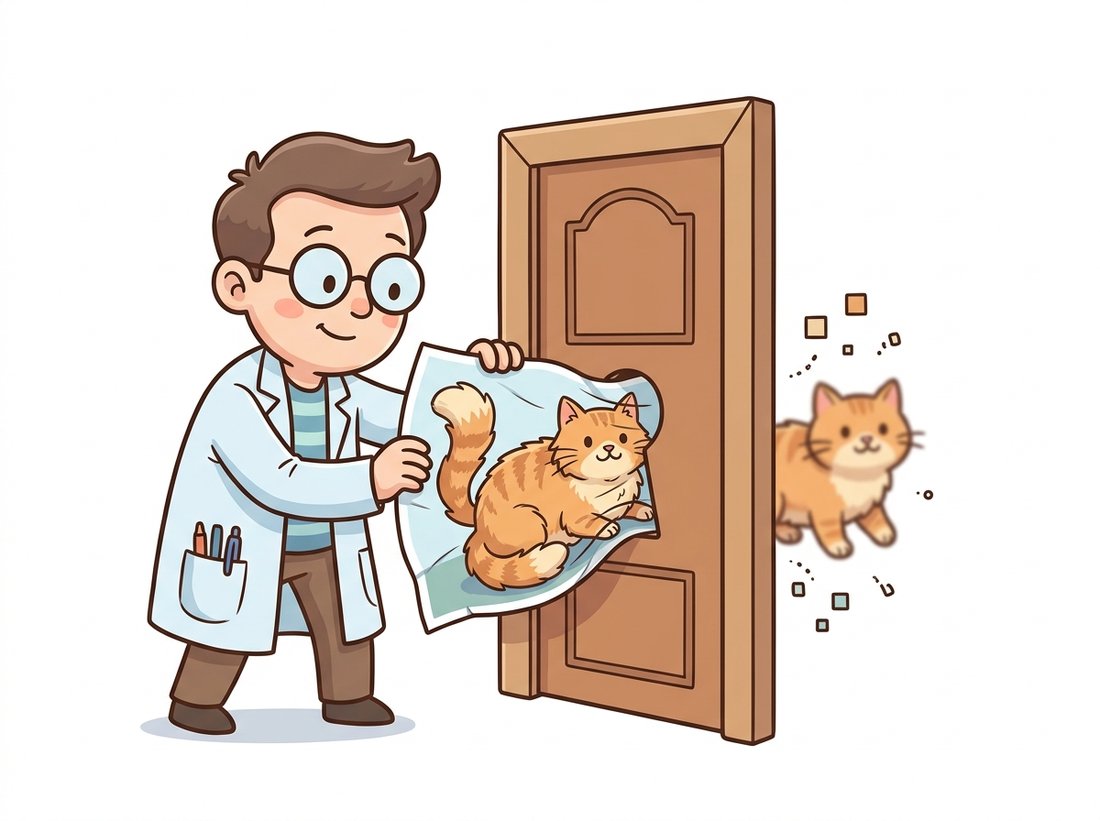
In the previous chapter you saw the landscape of generative models and the central role of the latent space, the low-dimensional surface that natural images cluster near inside their vast pixel space. This section gives you the first concrete way to find that surface, and it does so with an idea older and simpler than any generative theory: compression. You compressed images with classical transforms in Chapter 4, throwing away high-frequency coefficients that the eye barely notices. An autoencoder does the same thing, except it learns the transform from the data instead of fixing it in advance, and the transform it learns is tuned to the specific images it sees rather than to images in general. The illustration below captures the bottleneck in a single image.
1. The Encoder, the Bottleneck, and the Decoder Beginner
An autoencoder has three parts. An encoder $f$ maps an input $x$ (an image, flattened or kept as a tensor) to a code $z = f(x)$ that lives in a much smaller space. A decoder $g$ maps that code back to the input space, producing a reconstruction $\hat{x} = g(z)$. The code $z$ sits in the bottleneck, the narrowest layer of the network, and its dimension is the single most important design choice. Training minimizes a reconstruction loss that measures how close $\hat{x}$ is to $x$, most commonly the mean squared error
averaged over the training set. Nothing else is involved: no labels, no target other than the input itself. This is why the autoencoder is the purest example of self-supervised learning, where the supervision signal is manufactured from the unlabeled data. Figure 31.1.1 shows the hourglass shape that gives the architecture its name.
The code below implements precisely this for MNIST, whose images are $28 \times 28 = 784$ pixels. The encoder is a small multilayer perceptron that shrinks 784 inputs down to 32; the decoder mirrors it back up to 784 with a sigmoid so the outputs live in $[0, 1]$ like the normalized pixels. Read the two nn.Sequential stacks against the hourglass of Figure 31.1.1.
# Minimal undercomplete autoencoder for MNIST: an encoder MLP that
# funnels 784 pixels into a 32-dim bottleneck, and a decoder that mirrors
# it back. The forward pass returns both the reconstruction and the code.
import torch
import torch.nn as nn

class Autoencoder(nn.Module):
    def __init__(self, in_dim=784, code_dim=32):
        super().__init__()
        self.encoder = nn.Sequential(
            nn.Linear(in_dim, 256), nn.ReLU(),
            nn.Linear(256, 64), nn.ReLU(),
            nn.Linear(64, code_dim),          # bottleneck: 32-dim code
        )
        self.decoder = nn.Sequential(
            nn.Linear(code_dim, 64), nn.ReLU(),
            nn.Linear(64, 256), nn.ReLU(),
            nn.Linear(256, in_dim), nn.Sigmoid(),  # outputs in [0, 1]
        )

    def forward(self, x):
        z = self.encoder(x)        # compress
        x_hat = self.decoder(z)    # reconstruct
        return x_hat, z

model = Autoencoder()
x = torch.rand(8, 784)            # a batch of 8 flattened images
x_hat, z = model(x)
print("code shape:", z.shape)         # code shape: torch.Size([8, 32])
print("reconstruction shape:", x_hat.shape) # torch.Size([8, 784])Training is an ordinary supervised loop where the target happens to be the input. The next block runs it on real MNIST for a few epochs and reports the reconstruction error falling, which is the signal that the code is capturing more and more of each digit.
# Train the autoencoder on real MNIST as a self-supervised loop:
# the target is the input image itself, the labels are discarded, and
# the falling MSE signals that 32 numbers increasingly suffice per digit.
import torch
from torch.utils.data import DataLoader
from torchvision import datasets, transforms

tf = transforms.Compose([transforms.ToTensor(),
                         transforms.Lambda(lambda t: t.view(-1))])  # flatten to 784
train = datasets.MNIST("./data", train=True, download=True, transform=tf)
loader = DataLoader(train, batch_size=256, shuffle=True)

model = Autoencoder()
opt = torch.optim.Adam(model.parameters(), lr=1e-3)
loss_fn = nn.MSELoss()

for epoch in range(5):
    total = 0.0
    for x, _ in loader:                 # labels are ignored: self-supervised
        x_hat, _ = model(x)
        loss = loss_fn(x_hat, x)         # target IS the input
        opt.zero_grad(); loss.backward(); opt.step()
        total += loss.item() * x.size(0)
    print(f"epoch {epoch}: mse = {total / len(train):.4f}")
# epoch 0: mse = 0.0461
# epoch 1: mse = 0.0292
# ...
# epoch 4: mse = 0.0204It feels paradoxical that we train hard to reconstruct an image we already have and then throw the reconstruction away. The reconstruction is only a scorecard. Its quality tells us whether the code captured the input, but the prize is the code: a 32-dimensional vector that summarizes a digit. Once trained, you keep the encoder and use $z$ as a learned feature for clustering, retrieval, anomaly detection, or as the input to a smaller classifier. This separation of "the task we train on" from "the representation we keep" is the template for nearly all self-supervised learning in Chapter 25.
2. Why the Bottleneck Must Be Undercomplete Beginner
Why force the code to be small at all? Imagine the opposite: a code dimension equal to or larger than the input, an overcomplete bottleneck. Then the encoder and decoder can collude to learn the identity function, copying each pixel through untouched. Reconstruction is perfect, the loss is zero, and the code has learned nothing about the structure of digits; it is just the image again in a different layout. A code that perfectly reconstructs by memorizing is useless as a representation.
An undercomplete bottleneck (code dimension smaller than the input) makes the identity shortcut impossible. There are simply not enough numbers to store every pixel, so the network must spend its limited code budget on whatever is most reconstructable: the regularities shared across digits. It learns that strokes are continuous, that a digit has roughly one connected blob of ink, that certain pen movements are common and others never occur. The code becomes a description in terms of these regularities rather than in terms of raw pixels. The bottleneck width is therefore a knob on an explicit trade: too wide and the code memorizes, too narrow and the reconstruction degrades because genuine variation is being discarded. Table 31.1.1 shows the trade concretely on MNIST.
| Code dimension | Compression ratio | Reconstruction MSE | What it learns |
|---|---|---|---|
| 2 | 392:1 | 0.052 | Coarse digit identity only; reconstructions are blurry averages |
| 8 | 98:1 | 0.028 | Identity plus rough slant and thickness |
| 32 | 24.5:1 | 0.020 | Sharp digits with style; the sweet spot here |
| 784 | 1:1 (overcomplete) | ~0.000 | The identity function; the code is meaningless |
The two-dimensional code in the first row is special because you can plot it. The next block trains a code-2 autoencoder and scatters the codes of test digits, colored by their true label, to see whether the bottleneck has organized the digits without ever being told what a label is.
# Train a code-2 autoencoder and scatter the test-set codes colored by
# their true label. The labels are used only for coloring, never for
# training, so any clustering is evidence the bottleneck found structure.
import torch, matplotlib.pyplot as plt

ae2 = Autoencoder(code_dim=2)            # 2D bottleneck so we can plot it
# ... (train ae2 with the loop from subsection 1) ...

ae2.eval()
codes, labels = [], []
with torch.no_grad():
    for x, y in DataLoader(test_set, batch_size=512):
        _, z = ae2(x)
        codes.append(z); labels.append(y)
codes = torch.cat(codes).numpy()
labels = torch.cat(labels).numpy()

plt.scatter(codes[:, 0], codes[:, 1], c=labels, cmap="tab10", s=4)
plt.colorbar(label="true digit"); plt.title("2D autoencoder latent space")
plt.show()
# The 10 digit classes form loosely separated clusters,
# even though the network never saw a single label.Rerun the training loop with one line changed, code_dim set to 2, then 8, then 32, then 64, and watch two numbers each time: the final reconstruction MSE printed by the loop, and the visible sharpness of a few decoded test digits. Predict before you run that MSE will fall as the code widens, then check that the drop shrinks once you pass roughly 32, the point where extra capacity buys almost nothing on MNIST. That diminishing return is Table 31.1.1 turned into something you watched happen, and it is the clearest way to feel why the bottleneck width is the single most important knob in this section: too small and detail vanishes, too large and the code stops being a compression at all.
3. The Linear Case Is PCA Intermediate
There is a beautiful special case that anchors the autoencoder to classical statistics. Strip out the nonlinearities: let the encoder be a single linear map $z = W_e x$ and the decoder a single linear map $\hat{x} = W_d z$, and train with mean squared error. The optimal solution is then a familiar one. The subspace spanned by the decoder's columns is exactly the subspace of the top principal components of the data, the same principal component analysis you would get from the eigenvectors of the covariance matrix. A linear undercomplete autoencoder, in other words, learns to project onto the directions of greatest variance, which is the optimal linear compression in the squared-error sense. The two views agree for a simple reason. The variance a projection keeps and the squared error it discards always add up to the fixed total variance of the data, so keeping the most variance and losing the least reconstruction error are the same objective seen from two sides.
The formal statement is the Eckart-Young-Mirsky theorem. With centered data and covariance $\boldsymbol{\Sigma} = \tfrac{1}{N}\sum_i \mathbf{x}_i \mathbf{x}_i^\top = \mathbf{U}\boldsymbol{\Lambda}\mathbf{U}^\top$ and eigenvalues sorted $\lambda_1 \ge \lambda_2 \ge \cdots \ge \lambda_d$, the rank-$k$ linear map that minimizes the reconstruction error has decoder columns spanning $\operatorname{span}\{\mathbf{u}_1,\dots,\mathbf{u}_k\}$, the top-$k$ eigenvectors of $\boldsymbol{\Sigma}$, and the error it cannot avoid is exactly the discarded tail of the spectrum:
Any optimum is related to the principal axes by an invertible map of the code, so it spans the same top principal subspace rather than reproducing the eigenvectors exactly. Nonlinearity is precisely what lets a deep autoencoder beat this bound, following a curved manifold instead of a flat subspace.
This is worth holding onto for two reasons. First, it tells you what an autoencoder buys over PCA: the nonlinear encoder and decoder let it learn a curved low-dimensional surface rather than a flat subspace, which captures the genuinely nonlinear structure of images (a rotated digit traces a curve through pixel space, not a line). Second, it gives you a sanity baseline. If your fancy nonlinear autoencoder does not beat PCA's reconstruction at the same code dimension, something is wrong with your training. The next block makes the comparison directly.
# Sanity baseline: a 32-component PCA is the best LINEAR compressor at
# this code size. A trained nonlinear autoencoder should beat its
# reconstruction MSE; if it does not, the training is broken.
import torch
from sklearn.decomposition import PCA

# X_train: (N, 784) tensor of flattened MNIST, X_test similarly
pca = PCA(n_components=32).fit(X_train.numpy())
recon = pca.inverse_transform(pca.transform(X_test.numpy()))
pca_mse = ((X_test.numpy() - recon) ** 2).mean()
print(f"PCA-32 reconstruction MSE: {pca_mse:.4f}")    # PCA-32 reconstruction MSE: 0.0241

# A trained nonlinear autoencoder with the same 32-dim code should do better,
# because it can bend the latent surface to follow the data manifold.
print(f"Nonlinear AE-32 MSE: {ae_mse:.4f}") # Nonlinear AE-32 MSE: 0.0204When a linear projection is all you need, do not build and train a linear autoencoder; scikit-learn's PCA solves the same optimization in closed form via the singular value decomposition, with no gradient descent, no epochs, and no learning-rate tuning. The three lines PCA(n_components=32).fit(X).transform(X) replace roughly forty lines of model, loss, and training loop, and they handle the centering, the eigendecomposition, and the optimal component selection internally. Reach for the autoencoder only when you need the nonlinear surface that PCA cannot represent; for the linear case the closed-form solver is faster and exact.
Because the linear case recovers the PCA subspace, it is tempting to carry the full PCA intuition over and assume the trained code dimensions are ordered by importance (dimension 0 the "first component," capturing the most variance) and mutually orthogonal. They are not. PCA's closed-form solution returns components that are orthogonal and sorted by variance; a nonlinear autoencoder trained by gradient descent recovers only the same low-dimensional surface, with no preference for any particular set of axes inside it. The 32 code units are an arbitrary, entangled, unordered basis: deleting "dimension 0" does not remove the largest factor of variation, and two units may be strongly correlated. This is exactly why disentanglement (giving the axes individual meaning) is a separate, hard goal that Section 31.4 must pursue deliberately rather than something an autoencoder provides for free.
4. The Fatal Flaw: A Latent Space Full of Holes Intermediate
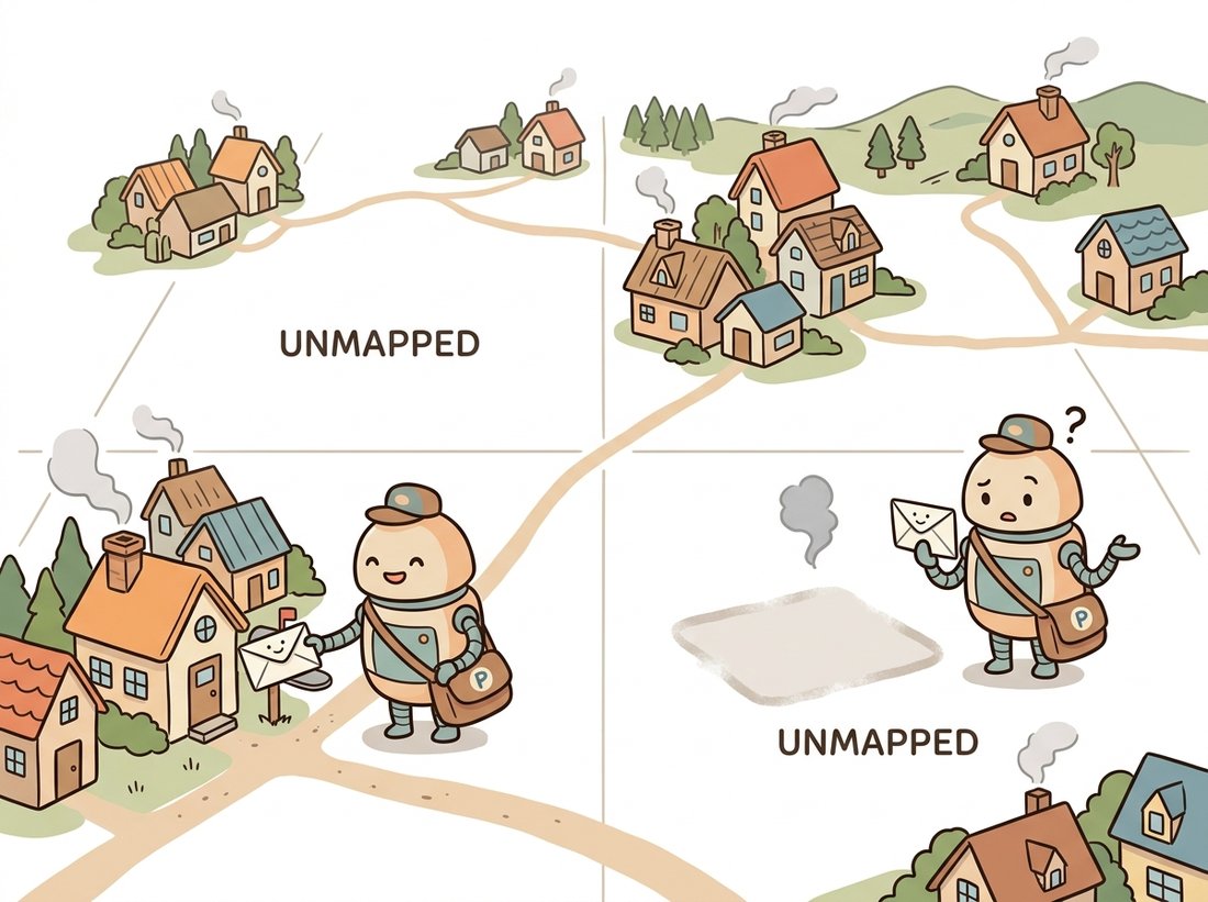
Now the catch that makes this whole chapter necessary. We have a generator-shaped object: an encoder, a decoder, and a low-dimensional code. It is tempting to think we can generate new digits by picking a random code $z$ and decoding it. We cannot, and the reason is structural. Nothing in the training objective ever asked the codes to fill the latent space in any particular way. The encoder is free to scatter the training codes wherever minimizing reconstruction is easiest, leaving large empty regions between clusters. Decode a point from one of those empty regions and you get an incoherent smear, because the decoder was never trained on anything that maps there. The illustration below makes the point with a postal-worker metaphor.
Two distinct problems live here. First, the codes have no fixed scale or shape, so you do not even know what range to sample from; the codes of subsection 2 might span $[-40, 40]$ in one axis and $[-2, 2]$ in another. Second, even sampling within the occupied range, you will frequently land between clusters where the decoder has never been trained, in a hole. Figure 31.1.2 contrasts the swiss-cheese latent of a plain autoencoder with the dense, fillable latent we want.
The experiment below makes the failure visceral. We sample a code from a standard normal (a perfectly reasonable guess for where codes might live) and decode it; the result is noise, because that code almost certainly fell in a hole.
# Show why a plain autoencoder cannot generate: sample a random Gaussian
# code and decode it. Because training never constrained where valid codes
# live, this code almost surely lands in a hole and decodes to a smear.
import torch

model.eval()
with torch.no_grad():
    z_random = torch.randn(1, 32)        # a guess at "a typical code"
    fake = model.decoder(z_random)       # decode it
print("output range:", fake.min().item(), "to", fake.max().item())
# output range: 0.41 to 0.58   <- a flat mid-gray band, no black ink or white paper
# Displaying `fake` shows an incoherent gray smear, not a digit.
# The plain autoencoder has no notion of which codes are "valid",
# so generation by random sampling fails. This is the gap the VAE closes.A plain decoder is less an artist than a postal worker. It knows how to deliver to the exact addresses the encoder ever wrote down during training, and at those addresses it does beautiful work. Hand it a random latitude and longitude in the empty ocean between the clusters and it shrugs and delivers a gray smear, because nobody lives there. The whole drama of the rest of this chapter is teaching the network to build a city with no vacant lots, so that wherever you knock, someone reasonable answers the door.
Who: a two-person team at a satellite-imagery startup, 2023. Situation: they trained a convolutional autoencoder to compress 512x512 multispectral tiles to a 256-dimensional code for cheap storage and fast similarity search, and it worked superbly, reconstructions were crisp and retrieval was fast. Problem: a product manager asked whether they could now "generate synthetic training tiles" by sampling codes, since they already had a decoder. The engineers tried it, sampled random codes, and got unusable static. Decision: rather than abandon the idea, they recognized the exact gap described in this subsection and converted the bottleneck to a variational one (the change of Section 31.3), accepting slightly softer reconstructions in exchange for a samplable latent. Result: the same architecture, now a VAE, produced plausible synthetic tiles useful for augmenting a scarce class, and the compression use case still worked. Lesson: a good autoencoder is a compressor by default and becomes a generator only when you constrain the latent space; the distinction is not architectural detail but the difference between a system that can and cannot sample.
The plain autoencoder never went away; it moved upstream. Every latent-diffusion system in 2024 to 2026, including the open Stable Diffusion 3.5 and SDXL lines, runs its diffusion process not on pixels but inside the latent space of a pretrained convolutional autoencoder (Hugging Face's AutoencoderKL), precisely because reconstructing from a compact code is cheap and the latent surface is smoother than pixel space. The frontier question is how aggressively you can compress before the decoder starts hallucinating detail: the "deep-compression autoencoder" (DC-AE; Chen et al., ICLR 2025, arXiv:2410.10733) pushed the spatial downsampling ratio far past the standard 8x, reaching 32x and reporting usable reconstruction up to 128x, to make high-resolution diffusion tractable, trading a harder-to-train autoencoder for a much cheaper diffusion stage. The bottleneck you built in this section is, quite literally, the front door of those systems. You will meet this autoencoder again as the compression stage of Chapter 33.
Explain in three or four sentences why an autoencoder whose code dimension equals the input dimension can drive its reconstruction loss to zero while learning nothing useful. Then describe a single change to the training setup (not the architecture) that could force even an overcomplete autoencoder to learn structure rather than the identity, and name which later section of this chapter formalizes that idea.
Train the code-2 autoencoder of subsection 2 on MNIST. Pick the codes of two test images of different digits, call them $z_a$ and $z_b$, and decode a sequence of ten interpolated codes $z_t = (1-t) z_a + t z_b$ for $t$ from 0 to 1. Display the ten decoded images in a row. Identify the values of $t$ at which the reconstruction becomes incoherent, and connect that incoherence to the "holes" of subsection 4: where along the straight line between two valid codes does the path leave the occupied region of the latent space?
Using the comparison code of subsection 3, measure the reconstruction MSE of PCA and of a nonlinear autoencoder at code dimensions 2, 8, 16, and 32 on the MNIST test set. Plot both curves on the same axes (MSE versus code dimension). At which code dimension is the nonlinear autoencoder's advantage over PCA largest, and at which is it smallest? Write a paragraph explaining the trend in terms of how much of MNIST's variation is genuinely linear versus how much requires the curved latent surface the nonlinear model can represent.