Denoising & Sparse Autoencoders

"Hand me a smudged photograph and I will tell you what it was supposed to be. I have seen ten thousand clean ones; the smudge is the only part I have never been allowed to keep."

A Denoising Autoencoder Who Has Made Peace With Noise

In Section 31.1 you built a plain autoencoder and saw that its undercomplete bottleneck forces the code to capture structure. This section keeps the encoder-decoder skeleton but swaps the constraint. Instead of relying on a narrow bottleneck, the denoising autoencoder uses a corruption process, and the sparse autoencoder uses an activation penalty. Both ideas predate deep learning's modern era, both turned out to matter far more than their inventors expected, and both connect directly forward to material later in this book. We take them one at a time.

1. The Denoising Autoencoder Beginner

The denoising autoencoder (DAE) changes one line of the training procedure. Before passing an image to the encoder, corrupt it: add Gaussian noise, set a random fraction of pixels to zero, or blur it. Crucially, the reconstruction target stays the clean original. The network sees $\tilde{x} = x + \text{noise}$ and is scored on how well its output $\hat{x}$ matches the uncorrupted $x$. The objective is

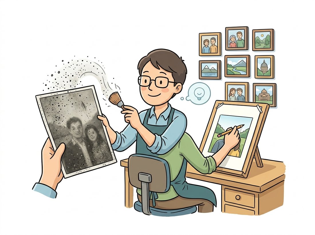
where $C$ is the corruption distribution. This is the classical denoising of Chapter 7 turned into a learning problem: where Chapter 7 hand-designed a Gaussian or non-local-means filter to remove noise, the DAE learns the denoiser from examples. To undo corruption the network cannot copy pixels through (the pixels are wrong); it must understand what a clean image looks like and project the noisy input back onto that manifold. That projection is exactly the structure we want the code to capture, and it is why a denoising autoencoder learns robust, transferable features even when its bottleneck is generous or absent. The illustration below casts the denoiser as an art-restorer who has seen thousands of clean examples.

There is a precise sense, not just a metaphor, in which this network learns the gradient of the data distribution. For Gaussian corruption $\tilde{x} = x + \sigma\varepsilon$, Vincent's denoising-score-matching identity (derived in full in Section 30.4) shows that the optimal denoiser's residual, rescaled, is exactly the score of the noised density:

In words: training a network to point a noisy sample back toward clean data is the same as training it to estimate which way density increases. That equivalence is the entire bridge to Chapter 33, where a denoiser run across a whole schedule of noise levels becomes a generative model; the DAE here is its single-noise-level ancestor.

The implementation reuses the encoder and decoder from Section 31.1 verbatim. The only change is that we add noise to the input inside the training loop while keeping the clean image as the target, as the comments in the next block make explicit.

# Denoising autoencoder: reuse the Section 31.1 architecture unchanged and
# alter only the training loop. Corrupt the input with Gaussian noise but
# score the output against the CLEAN original, forcing the net to denoise.
import torch
import torch.nn as nn

model = Autoencoder(code_dim=32)         # same architecture as Section 31.1
opt = torch.optim.Adam(model.parameters(), lr=1e-3)
loss_fn = nn.MSELoss()
noise_std = 0.4                          # corruption strength

for epoch in range(5):
    for x, _ in loader:                  # x is the CLEAN image, in [0, 1]
        x_noisy = (x + noise_std * torch.randn_like(x)).clamp(0, 1)  # corrupt
        x_hat, _ = model(x_noisy)        # encode/decode the CORRUPTED input
        loss = loss_fn(x_hat, x)         # but score against the CLEAN target
        opt.zero_grad(); loss.backward(); opt.step()
# At test time, feed a noisy digit and the DAE returns a clean one,
# having learned what "a digit" looks like rather than how to copy pixels.

The masking-noise variant, where a random fraction of input pixels are zeroed rather than perturbed, is worth a special mention because you have already met its descendant. Training a network to fill in missing pixels is exactly the pretext task of the Masked Autoencoder (MAE) from Chapter 25, which masks 75 percent of image patches and reconstructs them with a vision transformer. MAE is, in the most literal sense, a denoising autoencoder whose corruption is aggressive masking and whose backbone is a vision transformer. Figure 31.2.1 shows the corrupt-then-restore loop that unifies them.

2. The Sparse Autoencoder Intermediate

The sparse autoencoder takes the opposite tack from the bottleneck. Instead of making the code small, make it large, often larger than the input (overcomplete), but add a penalty that forces only a few code units to be active (nonzero) for any given input. The intuition is that each input should be explained as a combination of a handful of reusable parts drawn from a big dictionary, the way a face is a few specific features chosen from a vast catalog of possible features. The objective adds a sparsity term to the reconstruction loss:

where $\lVert z \rVert_1 = \sum_i |z_i|$ is the L1 norm of the code and $\lambda$ controls how aggressively sparsity is enforced. The L1 penalty is the same convexity trick that drives lasso regression: it pushes small activations exactly to zero rather than merely shrinking them, so the learned code is genuinely sparse, with most units off and a few strongly on. Because the constraint, not the dimension, does the regularizing, the bottleneck can be wide, and a wide-but-sparse code often learns more interpretable features than a narrow dense one. The next block adds the penalty to the training loop.

# Sparse autoencoder: make the code wider than the input (overcomplete)
# but add an L1 penalty so only a few units fire per image. The constraint,
# not a narrow bottleneck, is what now forces the code to learn structure.
import torch
import torch.nn as nn

class SparseAutoencoder(nn.Module):
    def __init__(self, in_dim=784, code_dim=1024):   # overcomplete: 1024 > 784
        super().__init__()
        self.encoder = nn.Sequential(nn.Linear(in_dim, code_dim), nn.ReLU())
        self.decoder = nn.Linear(code_dim, in_dim)

    def forward(self, x):
        z = self.encoder(x)
        return self.decoder(z), z

model = SparseAutoencoder()
opt = torch.optim.Adam(model.parameters(), lr=1e-3)
lam = 1e-3                                # sparsity weight lambda

for epoch in range(10):
    for x, _ in loader:
        x_hat, z = model(x)
        recon = ((x - x_hat) ** 2).mean()
        sparsity = z.abs().mean()         # L1 penalty drives most units to zero
        loss = recon + lam * sparsity
        opt.zero_grad(); loss.backward(); opt.step()
    frac_active = (z > 1e-3).float().mean().item()
    print(f"epoch {epoch}: active units = {frac_active:.1%}")
# epoch 0: active units = 41.2%
# ...
# epoch 9: active units = 6.8%   <- only a handful of the 1024 units fire per input

3. Sparse Autoencoders for Interpretability Advanced

For roughly a decade the sparse autoencoder was a respectable but minor member of the representation-learning toolkit. Then it found an unexpected and important second career. The problem it solves there is superposition: a trained neural network packs far more concepts into its activation vectors than it has neurons, so a single neuron lights up for many unrelated things and is impossible to interpret. The activations are dense and entangled. A sparse autoencoder trained on those activations learns to re-express each dense activation vector as a sparse combination of a much larger set of learned features, and those features turn out to be far more human-interpretable, one feature firing for "text in French," another for "the Golden Gate Bridge," another for a specific code pattern.

This is the technique behind the 2023 to 2024 wave of mechanistic-interpretability results, most prominently Anthropic's dictionary-learning work that recovered millions of monosemantic features from a production language model. The autoencoder is overcomplete by a large factor (tens of thousands of features for a few thousand activation dimensions), trained with exactly the L1 penalty of subsection 2, on the cached activations of a frozen model. The next block sketches the setup; the only conceptual change from subsection 2 is what the data is.

# The same sparse autoencoder, now aimed at interpretability: train it on a
# frozen model's cached activations with a large overcomplete factor so each
# learned feature becomes monosemantic (fires for one nameable concept).
import torch
import torch.nn as nn

# `acts` is a large tensor of cached activations from a frozen model,
# shape (num_tokens, d_model), e.g. d_model = 768.
class InterpSAE(nn.Module):
    def __init__(self, d_model=768, expansion=16):     # 16x overcomplete
        super().__init__()
        self.enc = nn.Linear(d_model, d_model * expansion)
        self.dec = nn.Linear(d_model * expansion, d_model)

    def forward(self, a):
        features = torch.relu(self.enc(a))   # sparse, interpretable feature set
        return self.dec(features), features

sae = InterpSAE()
# Train to reconstruct `acts` with a strong L1 penalty on `features`.
# After training, each large feature dimension tends to fire for ONE
# human-recognizable concept; inspecting the inputs that maximize a
# feature reveals what it detects. This is dictionary learning on a model's mind.