Energy-Based Models, Score Matching & Langevin Dynamics

"Nobody could tell me how much probability there was in total, so I gave up trying to count it. I only learned which way was uphill. Turns out that if you always know which way the data lies, and take small steps with a little luck mixed in, you arrive anyway. The grand total never mattered."

An Energy Function With a Missing Normalizer

The previous two sections took the latent route to $p(\mathbf{x})$: introduce a hidden code and decode it. This section takes a different route that uses no latent at all. We model the data distribution's shape directly through an energy, confront the partition-function problem that makes direct likelihood training impossible, and then sidestep it by learning the score and sampling with Langevin dynamics. This is the most mathematical section of the chapter, and it is deliberately so: the machinery here is the spine of modern diffusion, flagged in the cross-reference map as the arc that runs from energies and scores here, through the score SDEs of Chapter 33, to flow matching. We build it carefully so that arc feels like one continuous idea.

1. Energy-Based Models and the Partition Function Intermediate

An energy-based model (EBM) defines a probability density through a scalar energy function $E_\theta(\mathbf{x})$, a neural network that outputs one number per image. Low energy means high probability:

This is wonderfully flexible: any function $E_\theta$ at all defines a valid density, so the network has no architectural constraint (unlike the invertibility a flow demands). The catch is $Z_\theta$, the partition function, the normalizing constant that makes the density integrate to one. It is an integral over the entire $150{,}528$-dimensional image space, and it is hopeless to compute. Worse, it depends on $\theta$, so it changes every time we update the network. Maximum-likelihood training needs $\log p_\theta(\mathbf{x}) = -E_\theta(\mathbf{x}) - \log Z_\theta$, and the $\log Z_\theta$ term, with its intractable gradient, blocks the path. The energy view is the bottom of the cross-reference arc "scores and energies"; everything in this section is about getting useful behavior out of $E_\theta$ without ever touching $Z_\theta$.

2. The Score Is a Vector Field Pointing Toward Data Beginner

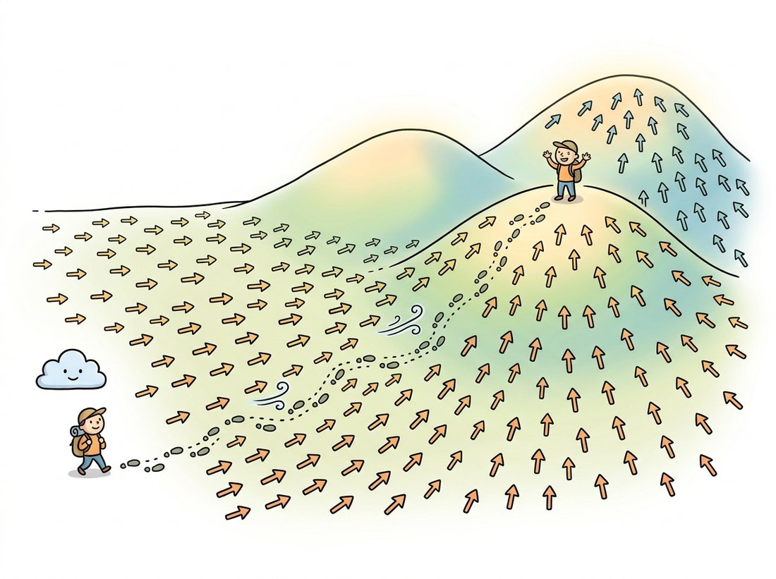
What is the score, geometrically? At every point $\mathbf{x}$ in image space, the score $\mathbf{s}(\mathbf{x}) = \nabla_{\mathbf{x}} \log p(\mathbf{x})$ is a vector pointing in the direction of steepest increase of log-probability, the direction that most quickly moves you toward more-probable images. Recall the manifold picture of Section 30.1: real images sit on a thin sheet, and almost everywhere else is low-probability noise. The score field is the set of arrows pointing back toward that sheet from wherever you are. Stand on a noise point and the score points toward the manifold; stand on the manifold and the score points along the directions of higher density. Figure 30.4.1 draws this field for a simple two-mode distribution.

3. Score Matching: Learning the Field Without the Density Advanced

This is the technical heart of the section, and it turns on a move that should feel impossible at first sight: we are about to fit a network to a target we can never observe. We want to train a network $\mathbf{s}_\theta(\mathbf{x})$ to match the true score $\nabla_{\mathbf{x}} \log p_{\text{data}}(\mathbf{x})$. The obvious objective, the expected squared difference between them, is unusable because we do not know the true score (it depends on the data density we are trying to learn). So how can you regress toward a quantity you never see? Hyvarinen's score matching result (2005) is the remarkable identity that answers it: that intractable objective equals, up to a constant, a tractable one that involves only the model's score and its derivative,

The true density never appears; only expectations over the data (which we approximate with samples) and the model's own score and Jacobian trace remain. (The trace term $\operatorname{tr}(\nabla_{\mathbf{x}} \mathbf{s}_\theta(\mathbf{x}))$ is the sum of the diagonal of the score's Jacobian, that is, how much each component of the score arrow grows as you nudge its own input coordinate; intuitively it rewards the field for spreading outward where data is dense.) The trace term is expensive in high dimensions, which led to two practical variants: sliced score matching (project the Jacobian onto random directions) and, far more important for vision, denoising score matching. The denoising variant adds Gaussian noise of scale $\sigma$ to the data and trains the network to predict the score of the noised distribution, which has a beautifully simple closed form: the score of a Gaussian-noised point is proportional to the noise that was added. That equivalence, learning the score equals learning to denoise, is the exact bridge to diffusion, and it is worth stating in code.

# Denoising score matching: add noise of scale sigma, predict the score.
# Key fact: for x_noisy = x + sigma * eps with eps ~ N(0, I),
#   the score of the noised density is  -(x_noisy - x) / sigma^2 = -eps / sigma.
# So a network that predicts the score is, up to scale, predicting the noise eps.
import torch
import torch.nn as nn

def denoising_score_matching_loss(score_net, x, sigma):
    eps = torch.randn_like(x)                       # the noise we add
    x_noisy = x + sigma * eps                       # corrupt the clean data
    target_score = -eps / sigma                     # closed-form score of the noised point
    pred_score = score_net(x_noisy, sigma)          # network's estimate of the score
    return ((pred_score - target_score) ** 2).mean()

# A tiny score network for a 2-D toy (in practice a U-Net over images).
score_net = nn.Sequential(nn.Linear(3, 64), nn.SiLU(),
                          nn.Linear(64, 64), nn.SiLU(),
                          nn.Linear(64, 2))
def net(x, sigma):                                  # concat sigma as a feature
    s = torch.full((x.size(0), 1), float(sigma))
    return score_net(torch.cat([x, s], dim=1))

x = torch.randn(256, 2)                             # toy "data" batch
loss = denoising_score_matching_loss(net, x, sigma=0.5)
print("DSM loss:", round(loss.item(), 4))           # DSM loss: a positive scalar to minimize

4. Langevin Dynamics: Sampling by Following the Score Advanced

A learned score field is a set of arrows; Langevin dynamics is how you turn arrows into samples. Starting from a random point, repeatedly take a small step in the score direction (uphill in probability) and add a calibrated dose of Gaussian noise:

The score term drags the sample toward high-density regions; the noise term keeps it from collapsing onto a single point and lets it explore. As the step size $\eta$ shrinks and the number of steps grows, the distribution of $\mathbf{x}_t$ provably converges to the true $p(\mathbf{x})$. Without the noise term this would be plain gradient ascent that piles every sample onto the nearest mode (no diversity); the noise is what makes it sample rather than optimize. The toy implementation below follows the score of a known two-mode density and shows the walk converging into the modes, exactly the red trajectory of Figure 30.4.1.

# Turn a known score field into samples by Langevin dynamics: from broad noise,
# repeatedly step uphill along the score and add a calibrated dose of Gaussian noise.
# Use a 1-D two-Gaussian mixture so the true score has a closed form to follow.
import torch

# Known toy density: mixture of two Gaussians in 1-D, so we can write the true score.
def true_score(x):
    # p(x) = 0.5 N(-2, 0.5^2) + 0.5 N(+2, 0.5^2); score = d/dx log p(x).
    import math
    def comp(mu): return torch.exp(-0.5 * ((x - mu) / 0.5) ** 2)
    pa, pb = comp(-2.0), comp(2.0)
    p = pa + pb                                       # unnormalized density (Z cancels in the score)
    grad = pa * (-(x + 2) / 0.25) + pb * (-(x - 2) / 0.25)
    return grad / p                                   # = d/dx log p(x)

def langevin(score_fn, n=2000, steps=500, eta=0.02):
    x = torch.randn(n, 1) * 3                          # start from broad noise
    for _ in range(steps):
        noise = torch.randn_like(x)
        x = x + 0.5 * eta * score_fn(x) + (eta ** 0.5) * noise   # the update above
    return x

samples = langevin(true_score)
# Most samples should land near -2 or +2, recovering the two modes.
near_a = ((samples + 2).abs() < 0.6).float().mean()
near_b = ((samples - 2).abs() < 0.6).float().mean()
print(f"fraction near mode -2: {near_a:.2f}, near +2: {near_b:.2f}")
# fraction near mode -2: ~0.49, near +2: ~0.49

One practical wrinkle drove the field forward. In high dimensions the score is poorly estimated far from the data (there is almost no training data out in the empty regions of pixel space), so naive Langevin sampling mixes badly. The fix, introduced by Song and Ermon in the Noise Conditional Score Network (2019), is to estimate the score at many noise levels and sample by annealed Langevin dynamics: start at a high noise level where the score is easy to estimate everywhere, then gradually anneal to low noise. That annealing across noise levels is, almost exactly, the reverse process of a diffusion model, which is why this section is the direct precursor to Chapter 33.

# Annealed score sampling, packaged. The scheduler bundles the noise-level
# schedule, step size, and noise injection that the hand-written langevin loop
# spelled out; sampling is a short loop over scheduler.timesteps (high to low noise).
import torch
from diffusers import UNet2DModel, DDPMScheduler

model = UNet2DModel.from_pretrained("google/ddpm-cifar10-32").to("cuda")   # a trained score/noise net
scheduler = DDPMScheduler.from_pretrained("google/ddpm-cifar10-32")        # the annealing schedule
scheduler.set_timesteps(1000)

x = torch.randn(4, 3, 32, 32, device="cuda")                               # start from pure noise
for t in scheduler.timesteps:                                              # high noise -> low noise
    noise_pred = model(x, t).sample                                        # the learned score/noise
    x = scheduler.step(noise_pred, t, x).prev_sample                       # one annealed update

5. The Hyvarinen Identity: Eliminating the Unknown Data Score Advanced

Section 3 stated score matching as a result and trusted you to take it on faith. We now earn it. The problem is sharp and worth restating before the solution: we want to minimize the Fisher divergence between the data score and the model score,

but the first term inside the norm, $\nabla_{\mathbf{x}} \log p_{\text{data}}(\mathbf{x})$, is exactly the quantity we cannot observe: the true score of the data distribution. The objective is well defined yet uncomputable, which is the wall that stops a naive regression dead. Hyvarinen's 2005 result is that this wall is an illusion. By expanding the square and applying integration by parts to one cross term, the unknown data score disappears entirely, leaving an objective in the model alone.

Expand the squared norm into three pieces:

The first piece does not contain $\theta$, so for optimization it is a constant we may discard. Its value is $\tfrac{1}{2}\,\mathbb{E}_{p_{\text{data}}}\|\nabla_{\mathbf{x}} \log p_{\text{data}}\|^2$, the self-energy of the data score; it is the price of admission we never have to pay because it never moves the minimizer. The third piece involves only the model and is harmless. Everything hinges on the middle piece, which still contains the unknown $\nabla_{\mathbf{x}} \log p_{\text{data}}$. Integration by parts is what removes it.

Work the 1-D case explicitly, where it is fully transparent; the multivariate version is the same argument applied coordinate by coordinate. Write $\psi(x;\theta) = s_\theta(x) = \tfrac{d}{dx}\log p_\theta(x)$ for the scalar model score. The cross term is

The data density has cancelled out of the integrand and now appears only through its derivative $\tfrac{d p_{\text{data}}}{dx}$. Apply integration by parts, $\int u'\,v = [uv] - \int u\,v'$, with $u = p_{\text{data}}$ and $v = \psi$:

The boundary term $[\,p_{\text{data}}\,\psi\,]_{-\infty}^{+\infty}$ vanishes under the mild regularity condition that $p_{\text{data}}(x)\,\psi(x;\theta) \to 0$ as $\|x\| \to \infty$, which holds whenever the data density decays at the tails faster than the model score grows (true for any density with finite variance and a reasonable model). What remains is $-\int p_{\text{data}}\,\tfrac{d\psi}{dx}\,dx = -\mathbb{E}_{p_{\text{data}}}\!\big[\tfrac{d}{dx}\psi(x;\theta)\big]$. The unknown data score is gone; only a derivative of the model score survives. Substituting back, and noting the cross term entered $J(\theta)$ with a minus sign, the two minus signs combine to a plus:

where in $d$ dimensions the parts integral runs once per coordinate and the surviving derivatives assemble into the trace of the Hessian of the log-density, $\operatorname{tr}(\nabla_{\mathbf{x}}^2 \log p_\theta) = \sum_i \partial^2/\partial x_i^2 \log p_\theta$, the Laplacian. This is exactly the objective of Section 3 (there written with the equivalent $\operatorname{tr}(\nabla_{\mathbf{x}} \mathbf{s}_\theta)$, since $\mathbf{s}_\theta = \nabla_{\mathbf{x}} \log p_\theta$), now derived rather than asserted. The dropped constant is the data-score self-energy $\tfrac{1}{2}\,\mathbb{E}\|\nabla \log p_{\text{data}}\|^2$ identified above; it shifts $J$ by a fixed amount but leaves $\arg\min_\theta J$ untouched, which is all an optimizer cares about.

6. Denoising Score Matching: A Closed-Form Target Advanced

The Laplacian term makes Hyvarinen's objective exact but costly, and the costlier it is the less it fits the high-dimensional vision setting that motivates this whole book. Vincent's 2011 denoising score matching removes the trace term entirely, at the price of a controlled approximation: instead of matching the score of the data, it matches the score of the data convolved with a small Gaussian. The trade is overwhelmingly worth it, because the convolution gives the regression target a closed form with no derivatives at all.

Perturb each clean point $\mathbf{x}$ with isotropic Gaussian noise, $q_\sigma(\tilde{\mathbf{x}}\mid\mathbf{x}) = \mathcal{N}(\tilde{\mathbf{x}};\,\mathbf{x},\,\sigma^2 \mathbf{I})$, and define the noised marginal $q_\sigma(\tilde{\mathbf{x}}) = \int q_\sigma(\tilde{\mathbf{x}}\mid\mathbf{x})\,p_{\text{data}}(\mathbf{x})\,d\mathbf{x}$. Vincent's theorem states that matching the score of this noised marginal is equivalent, up to a constant, to a denoising objective that uses only the per-sample conditional:

The target $\nabla_{\tilde{\mathbf{x}}} \log q_\sigma(\tilde{\mathbf{x}}\mid\mathbf{x})$ is the score of a single Gaussian centered at the known clean point, which we can write down in closed form. For $q_\sigma(\tilde{\mathbf{x}}\mid\mathbf{x}) \propto \exp\!\big(-\|\tilde{\mathbf{x}} - \mathbf{x}\|^2 / 2\sigma^2\big)$,

Read the target literally: it is the clean point minus the noisy point, scaled by $1/\sigma^2$, that is, it points from where you are ($\tilde{\mathbf{x}}$) back toward the clean data ($\mathbf{x}$). Since $\tilde{\mathbf{x}} = \mathbf{x} + \sigma\boldsymbol{\epsilon}$ with $\boldsymbol{\epsilon}\sim\mathcal{N}(\mathbf{0},\mathbf{I})$, this equals $-\sigma\boldsymbol{\epsilon}/\sigma^2 = -\boldsymbol{\epsilon}/\sigma$: the target is the negative of the added noise, scaled by $1/\sigma$, the opposite sign of the noise you injected. A network minimizing this loss is literally learning to point away from the noise it must remove, which is why denoising and score estimation are the same task. The code block of Section 3 (Code Fragment 1) implements exactly this target, $-\boldsymbol{\epsilon}/\sigma$; we have now derived where it comes from.

7. Noise-Conditional Networks and Annealed Langevin Sampling Advanced

Section 6 left us with a dilemma we could not resolve at a single noise scale: small $\sigma$ gives an accurate but poorly covered score, large $\sigma$ gives broad coverage but a biased score. Song and Ermon's 2019 Noise Conditional Score Network (NCSN) resolves it by refusing to choose. It trains one network $\mathbf{s}_\theta(\mathbf{x}, \sigma)$ conditioned on the noise level, over a geometric ladder $\sigma_1 > \sigma_2 > \dots > \sigma_L$ spanning from a large scale that fills the ambient space down to a small scale that resolves the data, and it learns the denoising-score target at every level simultaneously with a single weighted objective:

The bracket is the per-level denoising-score-matching loss of Section 6, with the target written as $-(\tilde{\mathbf{x}} - \mathbf{x})/\sigma_i^2 = (\mathbf{x} - \tilde{\mathbf{x}})/\sigma_i^2$ moved to the same side. The $\sigma_i^2$ weight is the load-bearing detail: the DSM target $(\mathbf{x} - \tilde{\mathbf{x}})/\sigma_i^2$ has typical magnitude of order $1/\sigma_i$, so its squared error scales like $1/\sigma_i^2$ and would let the smallest-noise level dominate the sum. Multiplying each term by $\sigma_i^2$ cancels that scaling and makes every level contribute a loss of order one, so the network allocates capacity evenly across the ladder rather than overfitting the low-noise end. This is the same weighting that reappears, under different names, in the loss-weighting design of diffusion training in Chapter 33.

With one network covering all noise levels, sampling resolves the coverage problem of Section 4 by walking down the ladder. The idea is annealed Langevin dynamics: run a short Langevin chain at the highest, easiest noise level, then use its endpoint to initialize the chain at the next level down, and repeat all the way to $\sigma_L$. Early levels move the sample into the right broad region of space (where high-noise scores are reliable everywhere); later levels sharpen it onto the data manifold (where low-noise scores are accurate). The per-level step size $\alpha_i = \epsilon\,\sigma_i^2/\sigma_L^2$ shrinks with the noise level so the chain takes large exploratory steps early and fine corrective steps late.

The update inside step (b) is the Langevin step of Section 4 with $\eta = \alpha_i$, now conditioned on the noise level and reusing the chain across levels. The block below implements the NCSN training objective: the weighted denoising-score-matching loss for a noise-conditional network, summed over the geometric ladder.

# NCSN training objective (Song & Ermon 2019): weighted denoising score matching
# for a noise-conditional network s_theta(x, sigma), summed over a geometric ladder.
# Per level the DSM target is (x - x_noisy) / sigma^2 = -eps / sigma; the sigma^2
# weight rescales each level's squared error to order one so no level dominates.
import torch

def ncsn_loss(score_net, x, sigmas):
    # x: (B, D) clean batch; sigmas: 1-D tensor of noise levels, large -> small.
    total = 0.0
    for sigma in sigmas:
        eps = torch.randn_like(x)                       # fresh noise per level
        x_noisy = x + sigma * eps                       # corrupt at this level
        target = (x - x_noisy) / sigma**2               # closed-form DSM score = -eps / sigma
        pred = score_net(x_noisy, sigma)                # noise-conditional score estimate
        per_level = 0.5 * ((pred - target) ** 2).sum(dim=1)   # squared error per example
        total = total + (sigma**2) * per_level.mean()   # sigma^2 weighting -> order-one terms
    return total / len(sigmas)

# Geometric noise ladder and a quick shape check on a 2-D toy batch.
sigmas = torch.exp(torch.linspace(0.0, -3.0, steps=10))    # 1.0 down to ~0.05, geometric
loss = ncsn_loss(lambda x, s: torch.zeros_like(x), torch.randn(256, 2), sigmas)
print("NCSN loss (zero net baseline):", round(float(loss), 4))   # a positive scalar to minimize

8. What You Carry Into the Diffusion Chapter Beginner

This section built the engine room of modern generation without ever naming diffusion as such. You learned that an energy defines a density up to an intractable constant; that the score, the gradient of log-probability, sidesteps that constant entirely; that the score can be learned by denoising; and that Langevin dynamics turns a learned score into samples, made robust by annealing across noise levels. When Chapter 33 introduces the forward noising process and the learned reverse process, you will recognize the reverse process as exactly the annealed score walk built here. The remaining foundational question is what we are actually trading when we choose one sampler or one family over another, the quality, diversity, and speed of the result, which is the subject of the next section.

References Advanced