Generative vs Discriminative: What Does It Mean to Model p(x)?

"A classifier and I were arguing. It said: tell me what is in the photo and I will tell you it is a cat. I said: tell me nothing, and I will hand you a cat that never existed. We are not the same. It got the easier job."

A Slightly Overconfident Generative Model

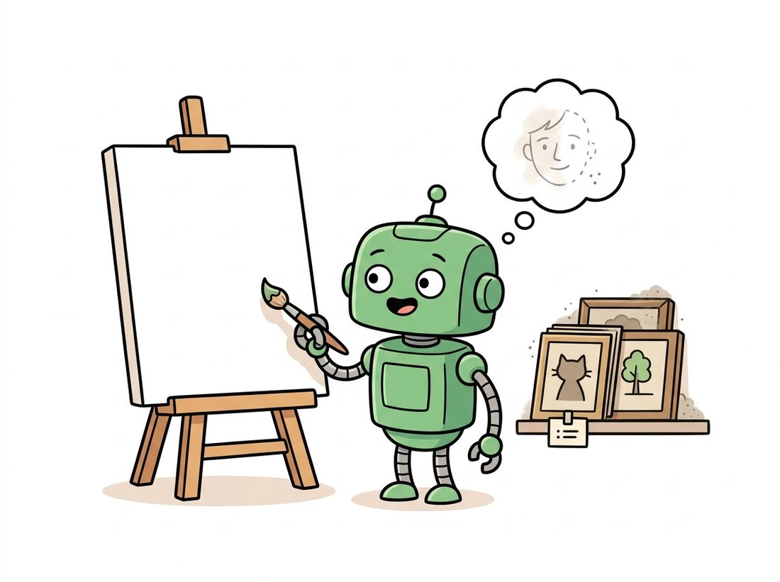
You arrive at this section having spent three parts of the book building discriminative models. Every classifier, detector, and segmenter you trained answered a question about an image that was handed to you. Now the image stops being the input and becomes the thing to be produced. This is the conceptual pivot of the entire generative part, and getting the framing right will pay off in every chapter that follows. We will define the two model types side by side, count the dimensions of the space a generator must conquer, see why almost all of that space is empty, and end with the concrete payoffs that motivate the whole enterprise. The next section, Section 30.2, then surveys the five families that attack $p(\mathbf{x})$ by different routes. The illustration below captures the whole pivot in one image: the job stops being to read a picture and becomes to imagine one.

1. Two Ways to Slice a Joint Distribution Beginner

Start from the joint distribution $p(\mathbf{x}, y)$ over images $\mathbf{x}$ and labels $y$. There are two ways to use it, and they correspond exactly to the two model types. A discriminative model learns the conditional $p(y \mid \mathbf{x})$ directly: given the pixels, what is the probability of each label? It never needs to know how images are distributed, only how to carve up the input space into label regions. A generative model learns $p(\mathbf{x})$, or the full joint $p(\mathbf{x}, y)$, which means it must model how the data itself is distributed. The two are linked by the chain rule and Bayes' rule:

A discriminative model takes the first factorization and learns only $p(y \mid \mathbf{x})$, treating $p(\mathbf{x})$ as someone else's problem. A generative classifier (such as a Gaussian mixture or a naive Bayes model) takes the second, learns $p(\mathbf{x} \mid y)$ and the prior $p(y)$, and recovers the label posterior by Bayes' rule. For pure generation, we drop $y$ entirely and model $p(\mathbf{x})$, the marginal over images. The crucial observation is that a model of $p(\mathbf{x})$ contains strictly more information than a model of $p(y \mid \mathbf{x})$: the former can draw samples, the latter cannot. Figure 30.1.1 contrasts the two geometrically.

2. The Curse of Pixel Space Intermediate

To feel why $p(\mathbf{x})$ is hard, count the dimensions. A single color image of height $H$, width $W$, and three channels is a point in $\mathbb{R}^{3HW}$. For a small $224 \times 224$ RGB image that is $3 \times 224 \times 224 = 150{,}528$ dimensions. A generative model must place a probability density over that entire space. If we naively discretized each of the $150{,}528$ values to its $256$ possible byte settings, the number of distinct images would be $256^{150528}$, a number so large that writing it out would exhaust the atoms in the observable universe many times over. The model has to assign almost all of its probability mass to the infinitesimal fraction of those arrangements that look like real photographs.

The following snippet makes the scale tangible by sampling pure noise, what a point chosen uniformly at random from pixel space actually looks like, and contrasting it with how few such draws will ever resemble anything.

# Count the dimensions of pixel space for a small RGB image, then draw one
# uniformly random point from it to see what an "average" image actually is.
# The point: real photos occupy a vanishing fraction of this space.
import numpy as np

H, W, C = 224, 224, 3
dim = H * W * C
print(f"pixel-space dimension: {dim:,}")          # pixel-space dimension: 150,528

# A point chosen uniformly at random from [0,255]^dim is "an image" too.
rng = np.random.default_rng(0)
random_image = rng.integers(0, 256, size=(H, W, C), dtype=np.uint8)
# Its per-channel histogram is flat: it is structureless static, not a photo.
print("mean:", random_image.mean().round(1), " std:", random_image.std().round(1))
# mean: 127.5  std: 73.9   <- exactly what uniform noise predicts

# The volume of "looks like a photograph" is a vanishing fraction of the whole.
# Modeling p(x) means concentrating density on that fraction.

This is the curse of dimensionality in its most extreme form: as the number of dimensions grows, the volume of the space explodes, points become almost uniformly far apart, and any finite dataset covers a vanishing fraction of the whole, so notions like distance and density that work well in two or three dimensions become nearly useless. The reason generative modeling is tractable at all is that natural images do not fill their space. They lie on (or very near) a much lower-dimensional surface inside it, the manifold of natural images, and the entire job of a generative model is to discover and describe that surface.

3. The Manifold of Natural Images Intermediate

The manifold hypothesis says that real data of a given type, photographs of faces, of streets, of handwritten digits, does not scatter through its high-dimensional ambient space but concentrates on a smooth, connected surface of far lower intrinsic dimension. A photograph cannot have arbitrary independent pixels: neighboring pixels are correlated, edges are continuous, lighting is globally consistent, objects obey geometry. Each such constraint removes degrees of freedom. The result is that a face image, nominally a point in $150{,}528$ dimensions, can in practice be described by a few hundred numbers: pose, identity, expression, lighting, background. Those few hundred numbers are the intrinsic coordinates of the face manifold. The illustration below makes the picture vivid: a sea of static with one thin shelf where actual photographs sit.

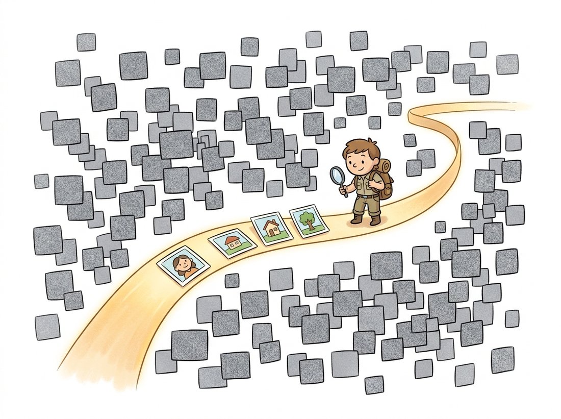
This picture, sketched in Figure 30.1.2, is the quiet protagonist of the whole part. The latent space we build in Section 30.3 is an attempt to parameterize this manifold directly, to find coordinates so that moving smoothly in latent space moves smoothly along the manifold of real images. The score of Section 30.4 is the gradient that points back toward the manifold from any off-manifold noise point, which is exactly what lets diffusion models in Chapter 33 walk a noise sample back onto the sheet. Holding the manifold picture in mind turns most of generative modeling from a bag of tricks into one coherent story.

4. What Modeling p(x) Buys You Beginner

Once a model holds $p(\mathbf{x})$, a striking range of capabilities becomes available from the single learned object. They divide into three families. First, sampling: draw a fresh $\mathbf{x} \sim p(\mathbf{x})$ and you have a new image that never existed, the core act of generation. Second, density evaluation: compute or estimate $p(\mathbf{x})$ for a given image and you can detect anomalies (low-probability inputs), compress (assign short codes to likely images), and compare models by held-out likelihood. Third, conditional inference: condition on partial or corrupted observations and sample the rest, which is exactly inpainting, super-resolution, denoising, and colorization, the classical restoration tasks of Chapter 7 reborn as draws from a conditional $p(\mathbf{x}_{\text{missing}} \mid \mathbf{x}_{\text{observed}})$.

The conditional case deserves emphasis because it unifies tasks that looked unrelated in earlier parts of the book. Inpainting fills missing pixels; super-resolution fills the high-frequency detail a low-resolution image lacks; denoising removes corruption; colorization fills the missing chroma channels. All four are the same operation under the generative lens: observe part of an image and sample the rest from the conditional distribution the generative model defines. We will see in Chapter 35 that controllable editing is this same conditional sampling with the conditioning made richer (a mask, a sketch, a text prompt). The toy below illustrates the simplest version, conditional sampling from a known two-dimensional density, so the idea is concrete before we scale it to images.

# A toy "data distribution": a ring of points (the manifold) in 2-D.
# Modeling p(x) here means knowing the ring; unconditional sampling draws on it,
# and conditional sampling observes one coordinate and completes the other.
import numpy as np

def sample_ring(n, radius=1.0, noise=0.05, rng=None):
    rng = rng or np.random.default_rng(0)
    theta = rng.uniform(0, 2 * np.pi, size=n)          # position along the manifold
    r = radius + rng.normal(0, noise, size=n)          # small off-manifold spread
    return np.stack([r * np.cos(theta), r * np.sin(theta)], axis=1)

data = sample_ring(2000)
print("data shape:", data.shape)                       # data shape: (2000, 2)

# Unconditional sample: just draw from p(x).
fresh = sample_ring(5)

# Conditional sample: observe x1 (say the left half) and complete x2.
# Given x1 = -0.5, the ring allows two completions: x2 = +/- sqrt(1 - x1^2).
x1 = -0.5
x2_options = np.array([+np.sqrt(1 - x1**2), -np.sqrt(1 - x1**2)])
print("completions of x1=-0.5:", x2_options.round(3))  # completions: [ 0.866 -0.866]

# Sample from a model that has already learned p(x) over a face dataset.
# from_pretrained downloads the trained weights; one pipeline call runs the
# full reverse sampling loop and returns a brand-new face image.
from diffusers import DDPMPipeline
pipe = DDPMPipeline.from_pretrained("google/ddpm-celebahq-256").to("cuda")
image = pipe(num_inference_steps=50).images[0]   # a fresh, never-seen face
image.save("sample.png")

5. Reading the Map Ahead Beginner

You now have the framing that the rest of Part IV builds on. Generation means modeling the distribution of the data rather than a boundary over it; that distribution lives in a colossal pixel space but concentrates on a thin manifold; and once learned it unlocks sampling, density evaluation, and conditional completion in one stroke. The natural next question is how, concretely, one represents and fits $p(\mathbf{x})$. There is no single answer, which is the point of the next section: five families have each found a different tractable handle on the intractable object $p(\mathbf{x})$. Section 30.2 lays them out side by side so you can see what each gives up and what each gains.