Latent Variables & the Idea of a Latent Space

"They told me I was three hundred numbers. I was insulted, until I learned that nudging the forty-second number put a smile on every face I decoded, and the eighty-first turned the lights to evening. Three hundred numbers, it turns out, is enough to hold a person. The trick was which three hundred."

A Latent Code Still Discovering Its Own Axes

In Section 30.2 three of the five families, VAE, GAN, and latent diffusion, all began the same way: draw a latent $\mathbf{z}$, then decode it to an image. That shared first move is the subject of this section. We will define what a latent-variable model is and the marginalization that connects the code to the image, build intuition for why a few hundred numbers can hold a whole picture, see the two operations (interpolation and latent arithmetic) that make latent spaces so useful for editing, and end on disentanglement, the open question of whether the axes of the latent space can be made to mean something. This is the conceptual groundwork that Chapter 31 turns into a trainable VAE and that Chapter 35 exploits for editing.

1. The Latent-Variable Model Beginner

A latent-variable model explains the observed data $\mathbf{x}$ through an unobserved (latent) cause $\mathbf{z}$. We specify two things: a simple prior $p(\mathbf{z})$ over codes, almost always a standard Gaussian $\mathcal{N}(\mathbf{0}, \mathbf{I})$, and a decoder $p_\theta(\mathbf{x} \mid \mathbf{z})$, a neural network that maps a code to a distribution over images. The model's distribution over images is then the marginal, obtained by integrating out the hidden code:

Read this as a recipe: to generate, sample a code $\mathbf{z} \sim p(\mathbf{z})$ from the simple prior, then push it through the decoder to get an image. The hard, multimodal distribution over pixels is built by warping a simple Gaussian through a flexible network. The latent dimension $d$ (the length of $\mathbf{z}$) is chosen far smaller than the pixel dimension, typically a few hundred against the hundred-and-fifty thousand of Section 30.1, which forces the decoder to discover the manifold's intrinsic coordinates rather than memorize pixels. Figure 30.3.1 shows the geometry: a Gaussian blob in latent space, warped by the decoder into the curved sheet of real images.

2. Why a Few Numbers Hold a Picture Beginner

It can feel implausible that two hundred and fifty-six numbers could encode a detailed face. The manifold hypothesis of Section 30.1 is the answer: a face is not an arbitrary array of pixels but a highly constrained object whose true degrees of freedom, identity, pose, expression, lighting, are few. The latent code is meant to carry those degrees of freedom, and the decoder supplies everything that is shared across all faces (that they have two eyes, that skin has texture, that shadows obey light). The representation-learning chapters of Part III already prepared you for this: in Chapter 25 a learned embedding vector summarized the semantic content of an image. The latent code is the same idea run in reverse, a vector you decode into an image rather than encode from one.

The snippet below makes the dimensions concrete and shows the single line that defines sampling for any latent-variable generator. The compression ratio it prints, image dimension over latent dimension, is a direct numerical statement of the manifold hypothesis at work.

# Build a minimal decoder that maps a 256-D latent code to a 64x64 color image,
# and confirm the compression ratio: a few hundred numbers stand in for ~12k pixels.
# Sampling is then one line: draw codes from N(0, I) and decode them.
import torch
import torch.nn as nn

latent_dim = 256
img_shape = (3, 64, 64)                       # a modest color image
img_dim = 3 * 64 * 64
print(f"latent dim {latent_dim}, image dim {img_dim}, "
      f"compression {img_dim / latent_dim:.0f}x")
# latent dim 256, image dim 12288, compression 48x

# A minimal decoder: latent vector -> image. The complexity lives in these weights.
decoder = nn.Sequential(
    nn.Linear(latent_dim, 4 * 4 * 256), nn.ReLU(),
    nn.Unflatten(1, (256, 4, 4)),
    nn.ConvTranspose2d(256, 128, 4, stride=2, padding=1), nn.ReLU(),   # 4 -> 8
    nn.ConvTranspose2d(128, 64, 4, stride=2, padding=1), nn.ReLU(),    # 8 -> 16
    nn.ConvTranspose2d(64, 32, 4, stride=2, padding=1), nn.ReLU(),     # 16 -> 32
    nn.ConvTranspose2d(32, 3, 4, stride=2, padding=1), nn.Tanh(),      # 32 -> 64
)

# Sampling is one line: draw from the prior, decode.
z = torch.randn(8, latent_dim)                # 8 codes from N(0, I)
images = decoder(z)                           # 8 images, shape (8, 3, 64, 64)
print("sampled batch:", tuple(images.shape))  # sampled batch: (8, 3, 64, 64)

3. Interpolation: Walking the Manifold Intermediate

Because the decoder is continuous and the latent space is smooth, you can interpolate: take two codes $\mathbf{z}_a$ and $\mathbf{z}_b$, walk along the path between them, and decode each waypoint. The result is a sequence of images that morphs smoothly from $\mathbf{x}_a$ to $\mathbf{x}_b$, every intermediate frame a plausible image rather than a pixel-wise crossfade. This is the clearest demonstration that the latent space has captured the manifold: a straight line between two real codes stays (approximately) on the manifold of real images.

One subtlety matters, and it is geometric. The Gaussian prior concentrates its mass on a thin shell at radius $\sqrt{d}$: each of the $d$ coordinates contributes roughly one unit of squared length, so a typical code has length near $\sqrt{d}$ and the exact center is vanishingly rare, counterintuitive but true once $d$ is large. A straight linear interpolation passes through that low-density center and can produce washed-out midpoints. Spherical linear interpolation (slerp) follows the great-circle arc on the shell instead, keeping every waypoint in a high-density region.

# Two ways to walk between two latent codes. lerp takes the straight chord and can
# dip through the empty center; slerp follows the great-circle arc on the Gaussian
# shell, keeping every waypoint in a high-density region the decoder handles well.
import torch

def lerp(z_a, z_b, t):
    """Straight-line interpolation; can dip through the low-density center."""
    return (1 - t) * z_a + t * z_b

def slerp(z_a, z_b, t):
    """Spherical interpolation along the Gaussian shell; stays in high-density region."""
    a = z_a / z_a.norm()
    b = z_b / z_b.norm()
    omega = torch.acos((a * b).sum().clamp(-1, 1))         # angle between the two codes
    so = torch.sin(omega)
    if so.abs() < 1e-6:                                    # codes nearly parallel
        return lerp(z_a, z_b, t)
    return (torch.sin((1 - t) * omega) / so) * z_a + (torch.sin(t * omega) / so) * z_b

z_a, z_b = torch.randn(256), torch.randn(256)
path = torch.stack([slerp(z_a, z_b, t) for t in torch.linspace(0, 1, 9)])
print("interpolation path:", tuple(path.shape))   # interpolation path: (9, 256)
# Decoding `path` yields 9 frames morphing smoothly from image A to image B.

4. Latent Arithmetic: Editing by Adding Vectors Intermediate

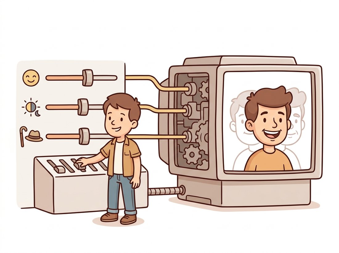
The second great trick is latent arithmetic. If a particular semantic attribute (smiling, wearing glasses, time of day) corresponds to a consistent direction in latent space, then adding a multiple of that direction to any code edits that attribute while leaving the rest of the image alone. The classic demonstration computed an "add a smile" vector as the difference between the average code of smiling faces and the average code of neutral faces; adding it to a frowning face's code produced a smiling version of the same person. Decode $\mathbf{z} + \alpha \, \mathbf{d}_{\text{smile}}$ for increasing $\alpha$ and you slide the expression from neutral to broad grin. This is the seed of all latent-space editing, and it is exactly what Chapter 35 scales up to inverting a real photo into a generator's latent space and editing it there. The illustration below shows the idea as a control panel: a few sliders feed a bulky decoder, and nudging one direction slides a single attribute.

# Edit an attribute by adding a vector. Estimate a semantic direction as the
# difference of group means (smiling minus neutral), then slide any code along it.
# In practice the group codes come from an encoder or from GAN inversion.
import torch

smiling_codes  = torch.randn(100, 256)          # codes of smiling faces
neutral_codes  = torch.randn(100, 256)          # codes of neutral faces

# An attribute DIRECTION is the difference of group means.
smile_dir = smiling_codes.mean(0) - neutral_codes.mean(0)
smile_dir = smile_dir / smile_dir.norm()        # unit direction

z = torch.randn(256)                            # the face we want to edit
edited = torch.stack([z + alpha * smile_dir     # slide along the smile axis
                      for alpha in torch.linspace(0, 3, 6)])
print("edit sequence:", tuple(edited.shape))    # edit sequence: (6, 256)
# Decoding `edited` shows the SAME identity gaining a progressively wider smile.

5. Disentanglement: Do the Axes Mean Anything? Advanced

Latent arithmetic works best when the latent space is disentangled: when distinct factors of variation (pose, identity, expression, lighting) are encoded along separate, independent directions, ideally aligned with the coordinate axes themselves. In a perfectly disentangled space, changing one coordinate would change exactly one human-meaningful property and nothing else. Real latent spaces are only partially disentangled; attributes are tangled together, so the smile direction may also slightly age the face. Methods such as the $\beta$-VAE (which up-weights the KL term in the ELBO to encourage independent latent coordinates) and StyleGAN's intermediate $\mathcal{W}$ space (a learned, less entangled latent than the input Gaussian) push toward disentanglement, and you will meet both later in the part. There is also a fundamental result that fully unsupervised disentanglement is impossible without some inductive bias or weak supervision, so the practical goal is a usefully structured space, not a perfectly factored one.

# Latent interpolation on a pretrained model: the starting noise tensor IS the
# latent code, so interpolate two seeds and run the deterministic DDIM denoiser
# on each waypoint to get a smooth morph, the slerp idea on a model that learned faces.
import torch
from diffusers import UNet2DModel, DDIMScheduler

model = UNet2DModel.from_pretrained("google/ddpm-celebahq-256").to("cuda")
scheduler = DDIMScheduler.from_pretrained("google/ddpm-celebahq-256")
scheduler.set_timesteps(50)

# The model's input noise IS its latent code; interpolate two seeds.
g = torch.Generator("cuda")
z_a = torch.randn(1, 3, 256, 256, generator=g.manual_seed(0), device="cuda")
z_b = torch.randn(1, 3, 256, 256, generator=g.manual_seed(1), device="cuda")

def denoise(latent):                                  # deterministic DDIM denoise
    x = latent.clone()
    for t in scheduler.timesteps:
        noise_pred = model(x, t).sample
        x = scheduler.step(noise_pred, t, x).prev_sample
    return x

frames = [denoise(torch.lerp(z_a, z_b, t))            # a 5-frame latent interpolation
          for t in torch.linspace(0, 1, 5)]

6. Why This Matters for the Whole Part Beginner

The latent space is the through-line of generative vision. It is the object the VAE learns to populate in Chapter 31, the space a GAN's generator reads from in Chapter 32, the compressed domain that latent diffusion operates in for efficiency in Chapter 33, and the canvas that editing tools manipulate in Chapter 35. Holding the three operations of this section, sample from the prior, interpolate along the manifold, and edit by adding directions, will let you read every one of those chapters as variations on a theme you already understand. The remaining foundational idea, how to learn the distribution when we refuse to use a latent and instead model the data's gradient field directly, is the energy and score view of the next section.