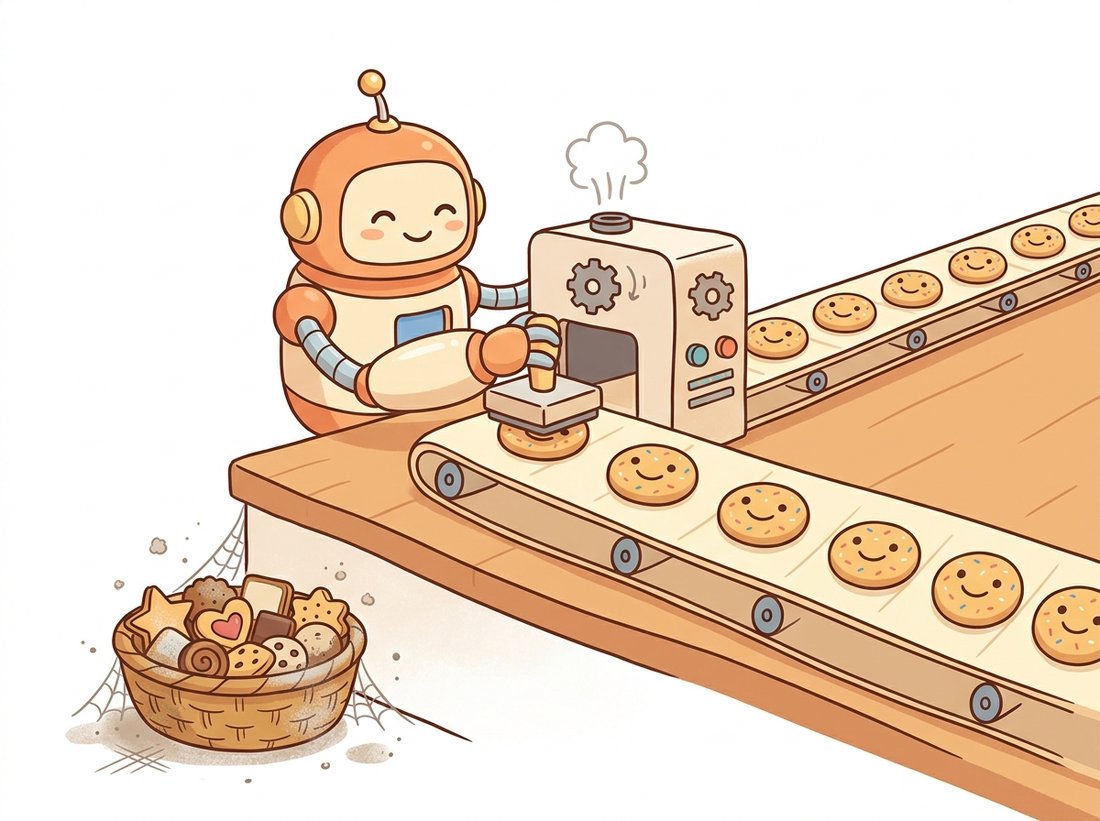
"I found one digit the bank could not tell from real, so I printed only that digit forever. They called it mode collapse. I called it efficiency. We were both, in our way, completely correct."
A Generator With Exactly One Good Idea
A GAN has no single loss to drive to zero; the healthy state is a balance between two networks, and most of the field's progress has been inventing ways to keep that balance from tipping over. This section names the three classic failure modes, mode collapse, vanishing gradients, and oscillation, and traces each to the geometry of the Jensen-Shannon divergence the original GAN minimizes. It then builds the two repairs that defined the late 2010s: the Wasserstein distance, which gives the loss a meaningful magnitude even when real and fake distributions barely overlap, and the Lipschitz constraints (gradient penalty, spectral normalization) that make the Wasserstein critic trainable. We close with the diagnostic habits that tell you, mid-run, whether your GAN is converging or quietly dying.
In Section 32.1 we derived a clean theory: at the global optimum the generator matches the data distribution and the discriminator is reduced to a coin flip. That theory assumes you can actually reach the optimum. In practice the two-player game is one of the hardest optimization problems in deep learning, because the thing you are descending keeps moving, and the surface it lives on has cliffs the moment the two distributions stop overlapping. This section is the honest middle of the chapter, the part the glossy sample grids never show.
1. The Three Classic Failures Intermediate
Mode collapse is the signature GAN failure. The data has many modes (ten digits in MNIST, thousands of object types in a photo dataset), but the generator discovers that producing just one or a few of them reliably fools the discriminator, so it abandons the rest. You see a sheet of nearly identical outputs. The cause is structural: the generator's objective rewards fooling the discriminator on the current batch, not covering the whole distribution, and nothing in the basic loss penalizes a generator for ignoring entire regions of $p_{\text{data}}$. If the discriminator catches up and learns to reject the over-produced mode, the generator simply hops to a different single mode, a behavior called mode hopping, and the two can chase each other around the data forever without the generator ever covering everything at once. The illustration below captures the spirit of it.
Vanishing gradients is the failure we previewed in Section 32.1. When the discriminator gets too good, it rejects fakes with near-certainty, and the gradient passed back to the generator shrinks toward zero. The non-saturating loss helps, but only partly: if the supports of $p_{\text{data}}$ and $p_g$ are disjoint, which is the generic situation early in training because both live on thin manifolds inside a huge pixel space, then an optimal discriminator can separate them perfectly and the Jensen-Shannon divergence is pinned at its maximum $\log 2$ regardless of how far apart they are. A constant divergence has zero gradient. The generator is told "you are wrong" but never "wrong in which direction".
Oscillation and non-convergence is the third. Because the two networks chase opposed objectives, the parameters can cycle indefinitely instead of settling, the discrete-time analogue of two players circling a saddle point. A famous toy example is a simple bilinear game whose continuous dynamics orbit the equilibrium forever; gradient descent on a GAN can do the same, with sample quality rising and falling in waves rather than improving monotonically. Figure 32.2.1 contrasts the three diseased loss patterns with the healthy one.
2. The Root Cause: Jensen-Shannon Has No Gradient When Supports Are Disjoint
The vanishing-gradient and the disjoint-support problems share one root, and seeing it clearly motivates everything that follows. Consider the simplest possible mismatch: $p_{\text{data}}$ is a point mass at $x = 0$ and $p_g$ is a point mass at $x = \theta$, and we slide $\theta$ from far away toward $0$. The Jensen-Shannon divergence between two non-overlapping point masses is the constant $\log 2$ for every $\theta \ne 0$, then drops discontinuously to $0$ at $\theta = 0$. (The Jensen-Shannon and KL divergences themselves were developed in Chapter 30.) As a function of the generator parameter $\theta$, the JSD is flat everywhere except at a single point, so its gradient is zero almost everywhere. No matter how the generator moves, the loss does not change, and gradient descent gets no signal about which direction reduces the gap.
This is not a quirk of point masses. Two distributions supported on low-dimensional manifolds inside high-dimensional pixel space almost never overlap, so the JSD between a real image distribution and a freshly initialized generator is generically pinned at its maximum. The discriminator can separate them perfectly, and a perfect discriminator gives no useful gradient. The clean theory of Section 32.1 assumed the optimum was reachable by gradient descent; this is the precise sense in which, with the original loss, it often is not.
The fix is to replace a distance that is constant when distributions do not overlap with one that decreases smoothly as they approach. For the point-mass example, you want a distance equal to $|\theta|$: it tells the generator exactly how far it has to go and in which direction. That distance is the Wasserstein, or earth mover, distance, and adopting it is the single most important stabilization in GAN history.
3. The Wasserstein GAN Advanced
The Wasserstein-1 distance $W(p_{\text{data}}, p_g)$ measures the minimum cost of transporting the mass of one distribution to match the other, where cost is mass times distance moved, hence the name "earth mover" (see the illustration below). For our two point masses it equals exactly $|\theta|$, which is the smooth, informative signal we wanted. The trouble is that the transport definition is an intractable optimization over all couplings (every possible plan for matching mass in one distribution to mass in the other). The Kantorovich-Rubinstein duality rescues it by proving that this same distance can be computed a completely different way, as a maximization over functions, which is something a neural network can do:
$$ W(p_{\text{data}}, p_g) \;=\; \sup_{\lVert f \rVert_L \le 1} \; \mathbb{E}_{\mathbf{x} \sim p_{\text{data}}} \big[ f(\mathbf{x}) \big] \;-\; \mathbb{E}_{\mathbf{x} \sim p_g} \big[ f(\mathbf{x}) \big], $$
where the supremum is over all 1-Lipschitz functions $f$ (functions whose output changes by at most the input distance). We approximate $f$ with a network, now called a critic rather than a discriminator because it outputs an unbounded real score instead of a probability. The critic maximizes the difference of its mean scores on real and fake images; the generator minimizes the negative of the critic's score on fakes. The whole objective becomes
$$ \min_{G} \max_{\lVert D \rVert_L \le 1} \; \mathbb{E}_{\mathbf{x} \sim p_{\text{data}}} \big[ D(\mathbf{x}) \big] \;-\; \mathbb{E}_{\mathbf{z} \sim p_z} \big[ D(G(\mathbf{z})) \big]. $$
There is no log and no sigmoid. Two consequences matter enormously in practice. First, the loss now means something: the critic's score difference is an estimate of the Wasserstein distance, so it correlates with sample quality and actually goes down as the generator improves, unlike the original loss whose magnitude told you almost nothing. Second, you can and should train the critic to near-optimality each step, because a better critic gives a better distance estimate rather than a vanishing gradient. The only catch is enforcing the $1$-Lipschitz constraint, which is what the next subsection is about.
4. Enforcing Lipschitz: Gradient Penalty and Spectral Normalization
The original Wasserstein GAN (WGAN) paper enforced the Lipschitz constraint by weight clipping, clamping every critic weight into $[-c, c]$ after each step. It worked but was brittle: too small a clip and the critic underfits, too large and the constraint is violated, and the clipped weights tend to pile up at the boundaries. Two cleaner mechanisms replaced it and remain standard.
Gradient penalty (WGAN-GP) notes that a function is $1$-Lipschitz exactly when its gradient has norm at most $1$ everywhere. Rather than clip weights, it adds a soft penalty that pushes the critic's gradient norm toward $1$, evaluated at random points $\hat{\mathbf{x}}$ interpolated between real and fake samples:
$$ \mathcal{L}_{\text{GP}} \;=\; \lambda \, \mathbb{E}_{\hat{\mathbf{x}}} \Big[ \big( \lVert \nabla_{\hat{\mathbf{x}}} D(\hat{\mathbf{x}}) \rVert_2 - 1 \big)^2 \Big], \qquad \hat{\mathbf{x}} = \epsilon \mathbf{x} + (1 - \epsilon) G(\mathbf{z}), \;\; \epsilon \sim U[0,1]. $$
The penalty weight $\lambda = 10$ is a robust default. The choice to evaluate the penalty at interpolated points $\hat{\mathbf{x}}$, rather than at the real or fake samples themselves, is deliberate: enforcing the Lipschitz constraint everywhere in image space is intractable, but the region between the two distributions is exactly where the critic builds the steepest slope that the generator must follow, so constraining the gradient norm there is both cheap (a single random point per image) and where it matters most. The implementation is short and is the reason WGAN-GP became the workhorse of the era.
# WGAN-GP Lipschitz enforcement: instead of clipping weights, softly
# push the critic's gradient norm toward 1 at random points interpolated
# between real and fake images, which keeps the critic 1-Lipschitz.
import torch

def gradient_penalty(critic, real, fake, device, lam=10.0):
    """WGAN-GP: penalize the critic's gradient norm away from 1
       at random interpolations between real and fake images."""
    bs = real.size(0)
    eps = torch.rand(bs, 1, 1, 1, device=device)          # one mix weight per image
    interp = (eps * real + (1 - eps) * fake).requires_grad_(True)
    scores = critic(interp)
    grads = torch.autograd.grad(
        outputs=scores, inputs=interp,
        grad_outputs=torch.ones_like(scores),
        create_graph=True, retain_graph=True)[0]            # create_graph: penalty is differentiable
    grads = grads.view(bs, -1)
    gp = ((grads.norm(2, dim=1) - 1.0) ** 2).mean()         # target gradient norm is exactly 1
return lam * gpcreate_graph=True, which makes the gradient-norm term itself differentiable so that backpropagation can flow through it into the critic's weights.Spectral normalization (Miyato et al., 2018) takes a different route. The Lipschitz constant of a linear layer is its largest singular value (spectral norm), and the Lipschitz constant of a composition is bounded by the product of the per-layer constants. So if you divide each layer's weight matrix by its own spectral norm, estimated cheaply with one step of power iteration per forward pass, every layer becomes $1$-Lipschitz and the whole critic is constrained for free. It adds almost no cost and is a single wrapper in PyTorch.
# Spectral normalization: divide each layer's weight by its largest
# singular value so every layer is 1-Lipschitz and the whole critic is
# constrained for free, with no extra loss term and negligible overhead.
import torch.nn as nn
from torch.nn.utils.parametrizations import spectral_norm

# Wrap each conv/linear in the discriminator; power iteration runs on the fly.
disc = nn.Sequential(
    spectral_norm(nn.Conv2d(3, 64, 4, 2, 1)), nn.LeakyReLU(0.2),
    spectral_norm(nn.Conv2d(64, 128, 4, 2, 1)), nn.LeakyReLU(0.2),
    spectral_norm(nn.Conv2d(128, 1, 4, 1, 0)),
)spectral_norm wrapper enforces a per-layer Lipschitz bound during every forward pass, with no extra loss term and negligible overhead.The two stabilizers above are exactly where libraries earn their keep. Spectral normalization from scratch means implementing power iteration, caching the estimated singular vectors across steps, and re-normalizing the weight on every forward pass, roughly thirty lines that are easy to get subtly wrong. PyTorch's torch.nn.utils.parametrizations.spectral_norm reduces all of that to a one-line wrapper per layer and handles the buffer management internally. Likewise the modern betas, two-time-scale learning rates, and exponential-moving-average of generator weights that production GANs rely on are built into training frameworks rather than re-derived each project.
5. Reading the Signs: GAN Diagnostics Intermediate
Because no loss curve tells the full story, diagnosing a GAN is a craft. A short checklist that catches most problems:
- Watch sample diversity, not just sample quality. The fastest mode-collapse detector is a fixed grid of latent vectors decoded every few epochs: if distinct $\mathbf{z}$ values start producing near-identical images, the generator is collapsing. Quantitatively, the Fréchet Inception Distance (FID) of Chapter 37 penalizes low diversity because it compares the full feature-distribution statistics, not individual images.
- Track the critic score gap. In a WGAN, the difference $\mathbb{E}[D(\text{real})] - \mathbb{E}[D(\text{fake})]$ is your distance estimate; it should shrink as training proceeds. A gap that grows without bound means the critic is overpowering the generator.
- Track $D(\text{real})$ and $D(\text{fake})$ in a standard GAN. Both near $0.5$ is healthy; $D(\text{real}) \to 1$ and $D(\text{fake}) \to 0$ means the discriminator is winning and the generator's gradient is vanishing.
- Save checkpoints often and keep the best by FID, not the last. Because runs oscillate, the final checkpoint is frequently worse than one from the middle of the run.
The one habit that separates people who can train GANs from people who cannot fits in five words: watch diversity, not the loss. A GAN loss curve can look perfectly healthy while the generator quietly prints the same image forever, which is exactly the trap that bit the medical team in the example below. Trust a fixed latent grid and FID, which both measure variety; treat the loss as a heartbeat, present means alive, but never as a quality score.
Learners meeting FID here often read it as a per-image quality score, so that a low FID guarantees each individual sample is sharp and a high FID means each is ugly. FID measures neither. It compares the distribution of Inception features over a large set of generated images against the same statistics over real images (the full definition is in Chapter 37), so it rewards matching the data's overall variety and statistics, not the prettiness of any one picture. The consequences matter for the failures in this section: a mode-collapsed generator that emits one flawless digit forever has low per-image quality variance but a terrible FID, because its feature distribution is far too narrow, which is precisely why FID catches the collapse a loss curve misses. The mirror trap is treating FID as ground truth for realism: it scores feature statistics, not semantics, so a set of plausible-looking but subtly wrong images can post a deceptively good FID. Use it to track diversity-plus-quality together, never as a verdict on a single sample.
Several light interventions rebalance a tipping game. Two time-scale update rules (TTUR) give the discriminator a higher learning rate than the generator, which the FID paper showed helps convergence to a local equilibrium. One-sided label smoothing replaces the real label $1$ with $0.9$ so the discriminator never becomes overconfident. Minibatch standard deviation, which we will meet in Section 32.3, feeds the discriminator a statistic of batch diversity so it can directly punish mode collapse. And simply training the critic multiple steps per generator step (five is the WGAN default) keeps the distance estimate accurate.
The instability of early GANs spawned an entire folklore of "GAN hacks", a widely circulated GitHub list of superstitions and tricks (normalize inputs to $[-1,1]$, use a spherical latent, avoid sparse gradients, flip labels occasionally) that practitioners traded like recipes. Many were never rigorously justified and some were later shown to be unnecessary once spectral normalization and good optimizers arrived, but for a few years the list was, only half-jokingly, the most-cited "paper" in the GAN community.
A research hospital team in 2019 wanted to augment a small, imbalanced dataset of dermoscopy images: melanomas were rare, and a classifier trained on the raw data missed them. The plan was to train a GAN to synthesize additional melanoma images and balance the classes. Their first model trained "successfully" by every loss they watched, both curves looked stable, but the augmented classifier got worse. The cause was severe mode collapse: the GAN had learned to reproduce a handful of training melanomas almost pixel for pixel, so the augmentation added thousands of near-duplicates of a few cases rather than genuine variety, and the classifier overfit to them. The team had been watching the wrong signal. Switching to a WGAN-GP critic, adding the minibatch-standard-deviation diversity statistic, and selecting checkpoints by FID rather than by loss produced a generator whose samples spanned the melanoma variety, and the augmented classifier's recall on held-out melanomas rose meaningfully. The lesson, repeated across the medical-imaging GAN literature, is that for any safety-critical use a GAN must be audited for memorization and diversity, never trusted on its loss curves alone.
Stabilization remains active research into the mid-2020s. NVIDIA's R3GAN (Huang et al., NeurIPS 2024) revisited the question of whether GANs are inherently unstable and argued no: with a well-posed regularized relativistic loss and a modern backbone, a plain GAN trains stably and competitively without the bag of tricks, challenging the folklore directly. On the conditional side, the discriminator-stabilization ideas here power the adversarial distillation of fast diffusion samplers (SDXL-Turbo in 2023, Stable Diffusion 3.5 Large Turbo in 2024), covered in Chapter 33, where the gradient-penalty and spectral-normalization lineage keeps the auxiliary discriminator well-behaved. The throughline is that the Lipschitz-control insight of Wasserstein GANs outlived the architecture that introduced it and is now infrastructure for the diffusion era.
Exercises
Using the two-point-mass example of Section 2, compute the Jensen-Shannon divergence and the Wasserstein-1 distance between a mass at $0$ and a mass at $\theta$, as functions of $\theta$. Sketch both. Explain in one paragraph why the Wasserstein curve gives a usable gradient for moving $\theta$ toward $0$ while the JSD curve does not, and connect this to the vanishing-gradient pathology.
Convert the MNIST GAN from Section 32.1 into a WGAN-GP: remove the sigmoid and BCEWithLogitsLoss, make the discriminator output a raw score (the critic), train the critic five steps per generator step, add the gradient_penalty function from this section, and use the Wasserstein losses (-critic(real).mean() + critic(fake).mean() + gp for the critic, -critic(fake).mean() for the generator). Log the critic's real-minus-fake score gap each epoch and confirm it decreases as samples improve, unlike the original BCE loss.
Deliberately induce mode collapse: take a working MNIST GAN and shrink the latent dimension to $2$, or train the generator far more often than the discriminator. Decode a fixed grid of $64$ latent vectors every five epochs and visually track diversity. Then estimate a crude diversity score (for example, the mean pairwise pixel distance among the $64$ samples) and plot it over training. Identify the epoch at which collapse begins, and describe which diagnostic from Section 5 would have flagged it earliest.