Section 32.3: DCGAN to StyleGAN: The Architecture Lineage

"They gave me a knob for every layer. One for the face shape, one for the hair, one for whether it is raining behind me. I did not ask for this much responsibility, but I will admit the portraits are spectacular."

A Style Vector With Too Many Dials

In Section 32.1 we built a GAN from fully-connected layers, and noted its samples were rough. In Section 32.2 we made training stable. This section is about capacity and control: how the generator's architecture evolved to produce high-resolution, high-fidelity images that you can also steer. The story spans roughly 2015 to 2020 and three landmark papers, and it is one of the clearest examples in deep learning of architecture, not just optimization, driving a capability jump.

1. DCGAN: The Recipe That Made GANs Trainable Beginner

The Deep Convolutional GAN (Radford et al., 2016) was less a new idea than a hard-won set of architectural rules that turned the temperamental original GAN into something a practitioner could reliably train. Its recipe is worth memorizing because variants of it underlie almost every convolutional GAN since. The generator is an all-convolutional network that upsamples a latent vector to an image; the discriminator mirrors it, downsampling an image to a score. The DCGAN rules are:

• Replace pooling with strided convolutions in the discriminator and transposed (fractionally-strided) convolutions in the generator, so both up- and downsampling are learned. These are the same transposed convolutions you used to upsample in the VAE decoder of Chapter 31.
• Use batch normalization (the per-batch activation rescaling of Section 19.4) in both networks (except the generator's output layer and the discriminator's input layer), which keeps activations well-scaled and was essential for deep stacks at the time.
• Remove fully-connected hidden layers; the architecture is convolutional end to end.
• Use ReLU in the generator (with Tanh at the output) and LeakyReLU in the discriminator, so the discriminator never fully zeroes a gradient.

Here is a compact DCGAN generator for $64 \times 64$ RGB images, exactly the structure used to produce the famous DCGAN bedroom and face samples.

# DCGAN generator for 64x64 RGB images: project the latent to a 4x4
# feature map, then upsample by 2 with transposed convolutions four times,
# following the DCGAN recipe (batch norm, ReLU, Tanh output).
import torch.nn as nn

class DCGANGenerator(nn.Module):
    def __init__(self, latent_dim=100, ngf=64, channels=3):
        super().__init__()
        self.net = nn.Sequential(
            # project the latent vector to a 4x4 feature map, then upsample x2 four times
            nn.ConvTranspose2d(latent_dim, ngf * 8, 4, 1, 0, bias=False),
            nn.BatchNorm2d(ngf * 8), nn.ReLU(True),               # 4x4
            nn.ConvTranspose2d(ngf * 8, ngf * 4, 4, 2, 1, bias=False),
            nn.BatchNorm2d(ngf * 4), nn.ReLU(True),               # 8x8
            nn.ConvTranspose2d(ngf * 4, ngf * 2, 4, 2, 1, bias=False),
            nn.BatchNorm2d(ngf * 2), nn.ReLU(True),               # 16x16
            nn.ConvTranspose2d(ngf * 2, ngf, 4, 2, 1, bias=False),
            nn.BatchNorm2d(ngf), nn.ReLU(True),                   # 32x32
            nn.ConvTranspose2d(ngf, channels, 4, 2, 1, bias=False),
            nn.Tanh(),                                            # 64x64, output in [-1, 1]
        )

    def forward(self, z):                  # z shape: (batch, latent_dim, 1, 1)
        return self.net(z)

DCGAN also gave the field its first vivid demonstration that the latent space is structured. Averaging the latent codes of "man with glasses" minus "man without glasses" plus "woman without glasses" decodes to a woman with glasses, the latent-arithmetic result that proved the generator had learned semantically meaningful directions. We exploit exactly this structure for editing in Section 32.5.

2. Progressive Growing: Coarse to Fine Intermediate

DCGAN topped out around $64 \times 64$. Pushing to $1024 \times 1024$ directly was unstable: a high-resolution discriminator can tell real from fake too easily on fine detail, and the generator cannot learn global structure and fine texture simultaneously from scratch. Progressive Growing of GANs (Karras et al., 2018) solved this with a training schedule rather than a new loss. Training begins at $4 \times 4$ with a tiny generator and discriminator. Once that stabilizes, a new layer is faded in to double the resolution, on both networks at once, with the new layer's contribution blended in gradually so the existing weights are not shocked. The process repeats up to the target resolution.

Progressive growing also introduced two small tricks that survived into later models: minibatch standard deviation, an extra discriminator feature that reports the variation across a batch so the discriminator can directly punish the low diversity of mode collapse (the diagnostic we flagged in Section 32.2), and equalized learning rate, which scales weights at runtime so every layer learns at a comparable pace. The result was the first GAN to produce $1024 \times 1024$ faces convincing enough to fool casual viewers.

3. StyleGAN: Style-Based Generation Advanced

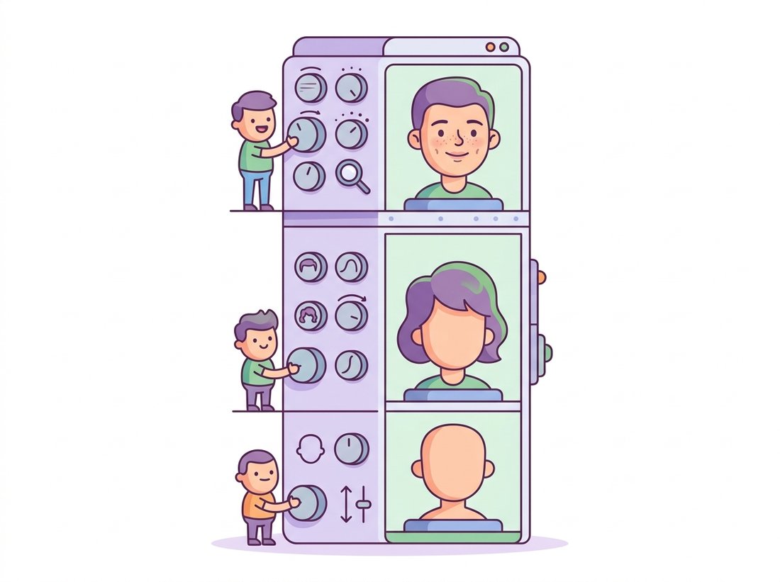
StyleGAN (Karras et al., 2019) kept progressive growing's training stability but redesigned the generator around a single question: can we control an image at multiple scales, coarse pose separately from fine texture? Its answer reshaped the field, sketched in the illustration below. Three architectural changes do the work.

A mapping network and the W space. Instead of feeding the latent $\mathbf{z}$ directly into the generator, StyleGAN first passes it through an eight-layer MLP that maps $\mathbf{z} \in Z$ to an intermediate vector $\mathbf{w} \in W$. The motivation is disentanglement: the prior $p_z$ is forced to be a fixed Gaussian, whose round shape cannot match the irregular distribution of real factors of variation, so $Z$ is necessarily entangled. The learned mapping network is free to warp $Z$ into a $W$ space whose geometry better matches the data, and empirically $W$ is far more disentangled. This is the space we will invert into in Section 32.5.

Style injection via adaptive instance normalization (AdaIN). The generator no longer takes a latent as its input at all. It starts from a learned constant $4 \times 4$ tensor, and the style vector $\mathbf{w}$ controls the image by modulating the statistics of every layer's activations. The intuition rests on a finding from style-transfer research: the per-channel mean and variance of a feature map encode its "style" (texture, color mood), so to apply a new style you erase the old statistics and write in new ones. At each layer, the feature map is instance-normalized (each channel set to zero mean and unit variance per image, the instance-normalization variant of Section 19.4), which strips the old style, then rescaled and shifted by a per-channel scale and bias predicted from $\mathbf{w}$, which writes the new one in:

$$ \mathrm{AdaIN}(\mathbf{x}_i, \mathbf{w}) \;=\; \mathbf{y}_{s,i}(\mathbf{w}) \cdot \frac{\mathbf{x}_i - \mu(\mathbf{x}_i)}{\sigma(\mathbf{x}_i)} \;+\; \mathbf{y}_{b,i}(\mathbf{w}), $$

where $\mathbf{y}_s$ and $\mathbf{y}_b$ are affine projections of $\mathbf{w}$. Because the same $\mathbf{w}$ feeds every layer, and because early (low-resolution) layers control coarse attributes while late (high-resolution) layers control fine ones, you can mix two images by using one $\mathbf{w}$ for the coarse layers and another for the fine layers, the celebrated style mixing that copies pose from one face and skin texture from another.

Per-layer noise for stochastic detail. Details with no semantic content (the exact placement of individual hairs, freckles, pores) are injected as explicit per-pixel Gaussian noise added at each layer, scaled by a learned per-channel factor. This frees the style vector from having to encode irreducibly random detail and is why two images with the same $\mathbf{w}$ but different noise differ only in their fine stochastic texture. Figure 32.3.2 contrasts the traditional and style-based generators.

A minimal style block makes the AdaIN mechanism concrete. The full StyleGAN generator stacks many of these at increasing resolution, but the core is just normalize-then-modulate.

# One StyleGAN synthesis layer: convolve, add learned-scale Gaussian noise,
# instance-normalize to strip per-channel statistics, then write new
# statistics back from the style vector w (adaptive instance normalization).
import torch
import torch.nn as nn
import torch.nn.functional as F

class StyleBlock(nn.Module):
    """One StyleGAN-style layer: conv, add noise, then AdaIN modulation from w."""
    def __init__(self, in_ch, out_ch, w_dim=512):
        super().__init__()
        self.conv = nn.Conv2d(in_ch, out_ch, 3, padding=1)
        self.noise_scale = nn.Parameter(torch.zeros(1, out_ch, 1, 1))   # learned per-channel
        self.to_style = nn.Linear(w_dim, out_ch * 2)                    # w -> scale and bias

    def forward(self, x, w):
        x = self.conv(x)
        x = x + self.noise_scale * torch.randn_like(x)                  # per-pixel stochastic detail
        x = F.instance_norm(x)                                          # zero mean, unit var per channel
        ys, yb = self.to_style(w).chunk(2, dim=1)                       # styles from the W vector
        return ys.unsqueeze(-1).unsqueeze(-1) * x + yb.unsqueeze(-1).unsqueeze(-1)

StyleGAN2 (Karras et al., 2020) refined this by replacing AdaIN with weight demodulation (folding the style into the convolution weights to remove characteristic "water-droplet" artifacts), dropping progressive growing in favor of a fixed skip-connection architecture, and adding path-length regularization to keep the mapping from $W$ to image smooth. StyleGAN2 is the model most GAN-inversion and editing work of Section 32.5 still builds on. StyleGAN3 then made the generator translation- and rotation-equivariant, removing the "texture sticking" that betrayed earlier models in video.

Exercises