Flow Matching, Rectified Flow & Consistency Models

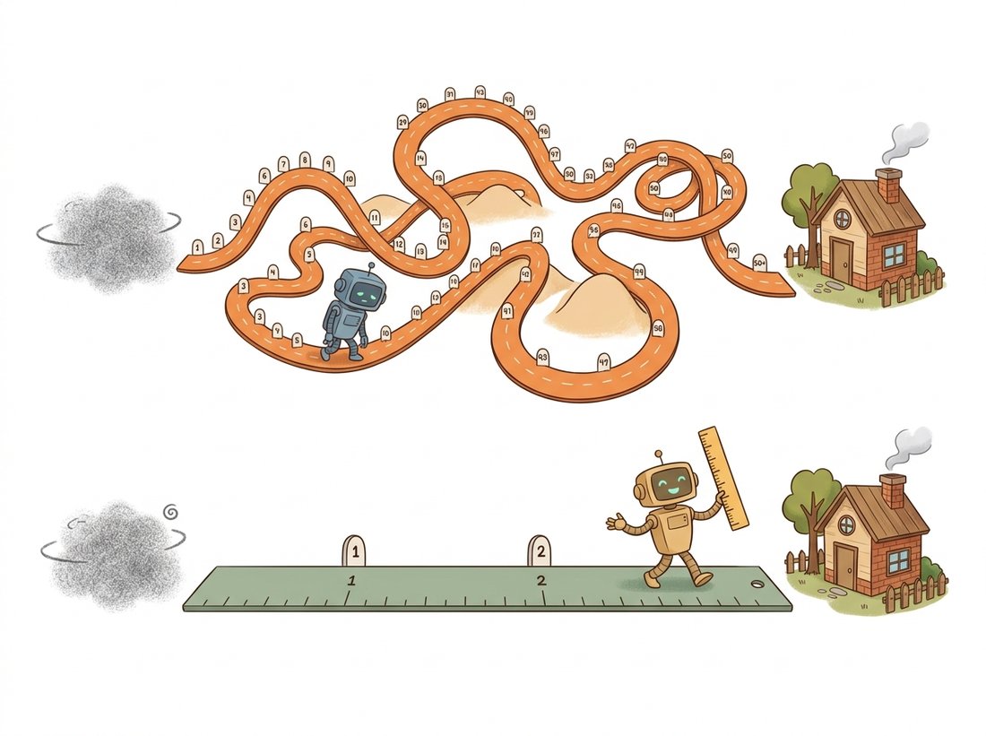
"Diffusion taught me to crawl from noise to data along a winding road. Flow matching handed me a ruler and said: why not walk in a straight line?"

A Velocity Field That Prefers the Shortest Path

The probability-flow ODE of Section 33.3 showed that a diffusion model is, at heart, an ODE whose velocity field carries noise to data, and Section 33.4 showed that the curviness of that field is what forces many sampling steps. The natural question is whether we can design a straighter field rather than inheriting the curved one that the diffusion forward process happens to produce. Flow matching answers yes, and gives a training objective for an arbitrary path that is simpler than the variational bound of Section 33.2. It is the modern descendant of the score-matching and energy-based view introduced in Chapter 30: where score matching learns the gradient of log-density, flow matching learns a velocity field directly, and the two meet in the probability-flow ODE. This section develops flow matching, specializes it to the straight-line rectified flow that modern systems use, and ends with consistency models, the most aggressive way to collapse the path to a single step.

1. Flow Matching: Learn the Velocity, Pick the Path Advanced

A continuous flow is defined by a time-dependent velocity field $v_\theta(x, t)$: to generate, you start at a noise sample $x_0 \sim \mathcal N(0, I)$ at time $t = 0$ and integrate $dx/dt = v_\theta(x, t)$ up to $t = 1$, landing on a data sample. Watch the subscripts here. Flow matching follows the convention that $t = 0$ is noise and $t = 1$ is data, so $x_0$ is the noise endpoint and $x_1$ is the data endpoint, the exact opposite of the diffusion chapters where $x_0$ was the clean image. Only the labels swap; the objects are the same. The question is how to train $v_\theta$ when we do not know the true velocity field. Flow matching's trick is to define the path between a specific noise sample $x_0$ and a specific data sample $x_1$ by a simple interpolation, and to regress the network onto the velocity of that conditional path, which we can compute. For the linear interpolation

The conditional flow matching loss simply asks the network to predict that velocity from the interpolated point and the time:

This is strikingly simple: draw a noise sample, draw a data sample, pick a random $t$, interpolate, and regress the network onto the constant velocity $x_1 - x_0$. There is no schedule of $\beta_t$, no variational bound, no closed-form posterior. A deep theorem (the one flow matching contributes) guarantees that minimizing this conditional objective also learns the correct marginal velocity field that transports the whole noise distribution to the whole data distribution. The same network you have been building all chapter, the time-conditioned U-Net or the transformer backbone of Chapter 22, plugs in unchanged; only the target and loss change. Figure 33.5.1 contrasts the curved diffusion path with the straight flow-matching path. The illustration below tells the same story as a journey: why wander a winding road when a ruler-straight one reaches the destination in a few strides?

The pair of functions below is the whole method: a loss that regresses the network onto the straight-line velocity, and a sampler that Euler-integrates the learned field from noise to data.

# Flow matching: train a velocity field on straight noise-to-data segments,
# then sample by Euler-integrating that field from t=0 (noise) to t=1 (data).
# There is no noise schedule and no variational bound, only a regression.
import torch

def flow_matching_loss(model, x1):
    """Conditional flow matching with linear (rectified-flow) paths.
    x1 is a batch of real data; x0 is sampled noise."""
    B = x1.size(0)
    x0 = torch.randn_like(x1)                       # noise endpoint
    t = torch.rand(B, *[1] * (x1.dim() - 1))        # uniform time, trailing 1s broadcast over image dims
    xt = (1 - t) * x0 + t * x1                       # straight-line interpolation
    target_velocity = x1 - x0                        # constant along the segment
    pred = model(xt, t.view(B))                      # flatten t to (B,) for the network; predict velocity
    return ((pred - target_velocity) ** 2).mean()

@torch.no_grad()
def flow_sample(model, shape, steps=10):
    """Generate by Euler-integrating the learned velocity field from t=0 to t=1."""
    x = torch.randn(shape)
    dt = 1.0 / steps
    for i in range(steps):
        t = torch.full((shape[0],), i * dt)
        x = x + model(x, t) * dt                      # straight Euler step
    return x

2. Rectified Flow: Straightening the Path Further Advanced

The linear interpolation in subsection 1 is straight for each individual noise-data pair, but the marginal field the network learns averages over all pairings and is generally still curved, because a given noise point is pulled toward many possible data points. Rectified flow fixes this with a reflow procedure: after training a first flow, generate noise-data pairs by actually running it, then retrain on those self-generated pairs. Because the pairs are now the ones the model itself transports, the optimal coupling becomes more straight-line, and after one or two reflow rounds the marginal trajectories are nearly straight. A straight marginal field is the holy grail for sampling: a straight line is solved exactly by a single Euler step. This is the theoretical reason a well-rectified flow can generate in one or two steps with quality that a diffusion model needs dozens to match. The architecture and the U-Net or diffusion transformer (DiT) denoiser are unchanged; rectification is a training-procedure refinement layered on the flow-matching loss.

3. Consistency Models: One Step to the Endpoint Advanced

Flow matching and rectified flow make the path straight; consistency models attack the problem from the other end by learning the solution map of the ODE directly. A consistency model $f_\theta(x_t, t)$ is trained so that for any point $x_t$ along a probability-flow trajectory (from Section 33.3), it outputs the trajectory's endpoint, the clean data, regardless of $t$. The defining property is self-consistency: two points on the same trajectory must map to the same endpoint, $f_\theta(x_t, t) = f_\theta(x_{t'}, t')$. This is enforced by a loss that pushes the model's output at one timestep to agree with its output (from an exponential-moving-average, or EMA, copy of itself) at an adjacent timestep along the trajectory. The boundary condition $f_\theta(x_0, 0) = x_0$ anchors the map. Once trained, generation is a single network call: feed pure noise, get a sample. Multi-step sampling is also available, alternate denoising to the endpoint and re-noising, to trade a few extra steps for quality. Consistency models can be trained from scratch (consistency training) or distilled from a pretrained diffusion teacher (consistency distillation), and the latter is how the fast Stable Diffusion variants of Section 33.4 are made.

4. The Continuity Equation and Why Conditional Flow Matching Works Advanced

Subsection 1 asserted that regressing on the easy conditional velocity also learns the correct marginal field. That claim is the engine of the whole method, and it deserves a proof rather than a promise. The starting point is the object we actually want. We want a velocity field $v_t(x)$ whose flow carries the noise distribution at $t=0$ into the data distribution at $t=1$. "Carries one distribution into another" has a precise meaning: as we push the points of a density along the field, the density must evolve consistently, with no probability mass created or destroyed. That conservation law is the continuity equation,

read as: the rate at which density piles up at a point ($\partial_t p_t$) equals the net inflow of the probability current $p_t v_t$ (the negative divergence). A field $v_t$ is said to generate the path $p_t$ exactly when this equation holds. The flow itself is the trajectory of an individual particle under that field, the ODE

so $\phi_t$ is the map that slides each starting point along the velocity field up to time $t$, and the marginal $p_t$ is the law of $\phi_t(x_0)$ when $x_0$ is drawn from the prior. If we knew the true generating field $u_t$, the obvious objective would be the marginal flow matching loss

This is intractable: we have no closed form for the marginal target $u_t(x)$, because $p_t$ is a mixture over every possible data point and computing $u_t$ at a single $x$ would require integrating against the whole data distribution. The Lipman et al. (2023) construction sidesteps the marginal entirely. Build the marginal path as a mixture of simple conditional paths, one per data point $x_1$:

where each conditional path $p_t(\cdot \mid x_1)$ is something we design to be trivial, a Gaussian that starts as the prior at $t=0$ and concentrates on $x_1$ at $t=1$, with a known conditional velocity $u_t(x \mid x_1)$ that generates it. The key lemma is that the marginal field generating $p_t$ is the conditional-velocity average weighted by the posterior over which data point produced $x$:

This is verified by substituting the mixture into the continuity equation: the marginal current $p_t(x) u_t(x)$ equals $\int p_t(x\mid x_1) u_t(x\mid x_1)\, q(x_1)\, dx_1$, the mixture of conditional currents, and since each conditional pair $(p_t(\cdot\mid x_1), u_t(\cdot\mid x_1))$ satisfies its own continuity equation, the integral satisfies the marginal one by linearity. So $u_t$ is a conditional expectation of $u_t(x\mid x_1)$ over the posterior.

5. Gaussian Conditional Paths and the OT Target Advanced

The lemma works for any family of conditional paths, so we get to choose the most convenient one. Pick a Gaussian conditional path that interpolates between the prior and a point mass on the data:

with the mean $\mu_t$ and standard deviation $\sigma_t$ chosen so that at $t=0$ the Gaussian is the standard prior and at $t=1$ it concentrates on $x_1$. We need the conditional velocity $u_t(x\mid x_1)$ that generates this Gaussian. A point on the path can be written as the reparameterization $x = \mu_t(x_1) + \sigma_t(x_1)\,\epsilon$ for a fixed standard-normal $\epsilon$; differentiating in time at fixed $\epsilon$ gives the velocity of that particle, $\dot x = \mu_t'(x_1) + \sigma_t'(x_1)\,\epsilon$. Eliminating $\epsilon = (x - \mu_t)/\sigma_t$ yields the closed-form conditional target

Each term is interpretable: the first scales the offset from the mean by the relative rate at which the Gaussian's width is changing (it contracts the cloud as $\sigma_t$ shrinks), and the second is simply the velocity of the mean itself. This single formula reproduces the targets of several known models depending on the schedule. The choice that yields the straightest individual trajectories, the optimal-transport (OT) path, takes the mean and width to be linear in time:

At $t=0$ this is $\mathcal{N}(0, I)$, the prior, and at $t=1$ it is $\mathcal{N}(x_1, \sigma_{\min}^2 I)$, a tight blob on the data point with a small floor $\sigma_{\min}$ that keeps the density well defined. Substituting $\mu_t' = x_1$ and $\sigma_t' = -(1-\sigma_{\min})$ into the general target gives

In the limit $\sigma_{\min} \to 0$ this collapses to $u_t(x\mid x_1) = (x_1 - x)/(1 - t)$, and along the path $x = (1-t)x_0 + t x_1$ the numerator $x_1 - x = (1-t)(x_1 - x_0)$ and denominator $1-t$ cancel to leave the constant $x_1 - x_0$. That recovers exactly the straight-line target of subsection 1: the linear interpolation and its constant velocity are the $\sigma_{\min}\to 0$ OT special case of the general Gaussian construction, now derived rather than asserted. The name "optimal transport" is earned because these straight, constant-speed conditional paths are the displacement-optimal interpolation between the two Gaussians under squared-Euclidean cost.

6. Rectified Flow as the Linear Special Case Advanced

Rectified flow (Liu et al., 2022) arrives at the same straight-line objective from a transport-first viewpoint rather than a probability-path one, and the equivalence is worth making explicit. Given any coupling of a noise sample $x_0$ and a data sample $x_1$, define the linear interpolation and regress the network on its (constant) time derivative:

This is identical to the CFM loss with the OT path at $\sigma_{\min}=0$; the constant target $x_1 - x_0$ is the conditional velocity of the straight segment, and the conditional-expectation argument of subsection 4 again guarantees the learned marginal field transports the noise marginal to the data marginal. The distinctive contribution of rectified flow is what it does after this first fit. The marginal field learned from an arbitrary (typically independent) coupling is straight for each pair but curved on average, because a single noise point is regressed toward many different data points and learns their average direction, which bends. Reflow repairs this: simulate the trained ODE from many noise samples to obtain the data points it actually produces, forming a new deterministic coupling $(x_0, \Phi(x_0))$, then refit the linear objective on these self-generated pairs. The new coupling never sends two trajectories through the same point in different directions, so its marginal interpolant has lower transport cost and is provably straighter; iterating drives the trajectories toward genuinely straight lines that a single Euler step solves exactly. One reflow round is usually enough to make few-step sampling work, and the procedure is the reason the title of the paper is "Flow Straight and Fast."

7. Consistency Models: Parameterization and the Distillation Loss Advanced

Subsection 3 described self-consistency in words; here is the construction that makes it trainable. A consistency model must satisfy two requirements simultaneously, and naive networks satisfy neither for free. First, the boundary condition: at the smallest time $\epsilon$ the map must be the identity, $f_\theta(x, \epsilon) = x$, because a point already at the trajectory's clean end has nothing left to denoise. Second, self-consistency across the trajectory, $f_\theta(x_t, t) = f_\theta(x_{t'}, t')$ for any two times on the same probability-flow ODE path of Section 33.3. The boundary condition is enforced by construction through the parameterization

where $F_\theta$ is the raw network. The skip coefficient $c_{\text{skip}}$ carries the input straight through and the output coefficient $c_{\text{out}}$ scales the network's correction; at $t=\epsilon$ the constraints force $f_\theta(x,\epsilon) = 1\cdot x + 0\cdot F_\theta = x$ automatically, no matter what $F_\theta$ outputs. Away from the boundary $c_{\text{skip}}$ falls and $c_{\text{out}}$ rises so the network does the work. This is the same skip-plus-output design used by the EDM preconditioning of Section 33.4, reused here to bake in the identity at $\epsilon$ rather than to normalize the loss scale.

Self-consistency is then trained, not constructed, by a loss that ties the model's outputs at two adjacent points on the same trajectory. Take a fine time grid $\epsilon = t_1 < t_2 < \cdots < t_N = T$. Draw a data point, noise it to level $t_{n+1}$ to get $x_{t_{n+1}}$, and take one ODE solver step backward to the adjacent level $t_n$ using the probability-flow field (the teacher's score in distillation), producing $\hat x_{t_n}$. The consistency distillation loss asks the model at $t_{n+1}$ to match a frozen copy of itself at the neighboring $t_n$:

where $d(\cdot, \cdot)$ is a distance (squared $\ell_2$, $\ell_1$, or LPIPS), $\lambda(t_n)$ is a positive per-step weight, and $\theta^- = \text{stopgrad}\big(\text{EMA}(\theta)\big)$ is a target network that is the exponential moving average of $\theta$ with the gradient detached. Three design choices make this work. The target $\hat x_{t_n}$ is produced by one ODE step from $x_{t_{n+1}}$, so the two arguments lie on a common trajectory and self-consistency is exactly what the loss measures. The stop-gradient prevents the trivial collapse in which the model drives both sides to a constant. The EMA target supplies a slowly moving, stable regression goal, the same stabilization idea as the target networks of value-based reinforcement learning. Because the boundary condition pins $f_\theta(\cdot,\epsilon)$ to the identity and the data point is the true endpoint at $t_1=\epsilon$, the chain of pairwise agreements propagates the correct endpoint all the way up the trajectory: minimizing $\mathcal{L}_{\text{CD}}$ to zero makes $f_\theta(x_t, t)$ return the trajectory's clean endpoint from any $t$, which is precisely the one-step generator. Consistency training replaces the teacher's ODE step with an unbiased single-sample estimate of the score, removing the need for a pretrained model at the cost of a noisier target.

# Rectified-flow training step and Euler ODE sampling, with the explicit
# constant target x1 - x0. Convention: t=0 is noise, t=1 is data.
import torch

def rectified_flow_step(model, x1, opt):
    """One optimization step of the rectified-flow / CFM-OT objective."""
    x0 = torch.randn_like(x1)                          # noise endpoint x0 ~ N(0, I)
    t  = torch.rand(x1.size(0), *[1] * (x1.dim() - 1)) # uniform t in [0, 1)
    xt = (1 - t) * x0 + t * x1                          # linear interpolation point
    target = x1 - x0                                    # constant velocity of the segment
    pred = model(xt, t.view(x1.size(0)))               # network predicts the velocity
    loss = ((pred - target) ** 2).mean()               # least-squares -> learns marginal field
    opt.zero_grad(); loss.backward(); opt.step()
    return loss.item()

@torch.no_grad()
def euler_sample(model, shape, steps=4):
    """Sample by Euler-integrating dx/dt = v_theta(x, t) from t=0 to t=1."""
    x = torch.randn(shape)                              # start at noise
    dt = 1.0 / steps
    for i in range(steps):
        t = torch.full((shape[0],), i * dt)
        x = x + model(x, t) * dt                        # straight Euler step
    return x                                            # lands near the data manifold