Latent Diffusion: Compress First, Then Diffuse

"Why repaint every blade of grass when a small map of the meadow will do? Compress the world, dream in the compressed world, and only render it back to pixels when someone insists on looking."

A Latent Vector That Saved Everyone a Fortune in GPU Hours

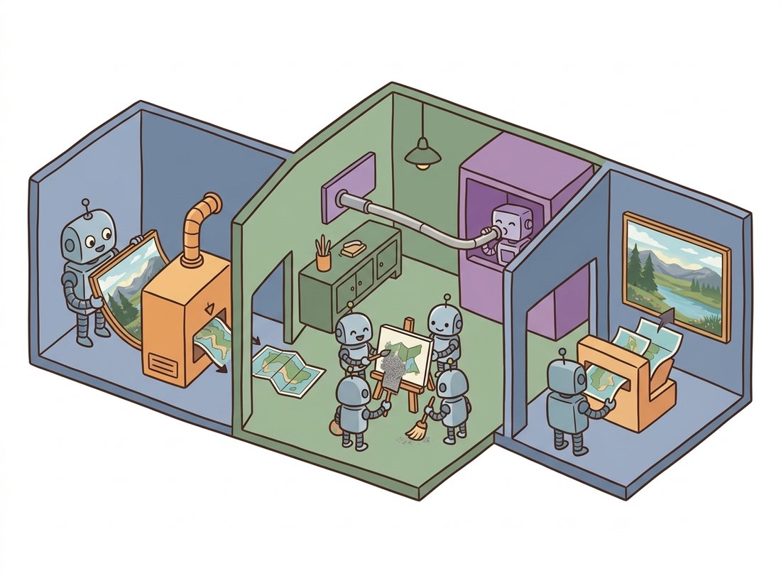
Every diffusion model in this chapter so far has operated on pixels: the noisy $x_t$ is a full-resolution image, and the U-Net processes it at that resolution at every one of the sampling steps. For a 512x512 RGB image that is roughly 786,000 numbers per step, and the compute of a convolution scales with that count. Pixel-space diffusion at high resolution is therefore enormously expensive, which is why the early models were trained by large labs on big clusters. Latent diffusion (Rombach et al., 2022), the model the world knows as Stable Diffusion, removes that wall with one idea borrowed from Chapter 31: do the diffusion in a compressed latent space instead. This section builds the two-stage system, explains why splitting perception from generation works, and ends with the diffusion transformer backbone that now scales the idea to video and beyond. The illustration below walks through the pipeline as a three-room workshop: compress, dream in the small space, then render once.

1. Two Stages: Perceptual Compression, Then Generation Intermediate

Latent diffusion factors the problem into two independently-trained stages. The first stage is an autoencoder (specifically a VAE-style encoder-decoder, often with a small adversarial and perceptual loss to keep decoded images sharp) that learns to compress an image into a much smaller latent tensor and reconstruct it. A typical Stable Diffusion autoencoder maps a 512x512x3 image to a 64x64x4 latent, an eightfold spatial downsampling and a roughly 48-fold reduction in element count (the spatial grid shrinks by $8 \times 8 = 64$ while the channels grow from 3 to 4, and $64 \times 3/4 = 48$). Crucially, this autoencoder is trained once and then frozen; it is a fixed perceptual codec. The second stage is the diffusion model from the rest of this chapter, but trained entirely on these latents: the forward process noises the latent, and the denoiser learns to predict the noise in latent space. At generation time you run diffusion in the latent, then decode the final latent to pixels once. Figure 33.7.1 shows the full pipeline with conditioning wired in.

The training step below makes the two-stage structure concrete: a frozen autoencoder encodes the image to a latent, and the conditional U-Net learns to predict the noise added in that latent space.

# Latent diffusion training step using pretrained diffusers components.
# A frozen VAE encodes the image to a small latent; the diffusion loss
# then runs in that latent space exactly as in the pixel-space version.
import torch
from diffusers import AutoencoderKL, UNet2DConditionModel, DDPMScheduler

vae = AutoencoderKL.from_pretrained("stabilityai/sd-vae-ft-mse")   # frozen codec
unet = UNet2DConditionModel.from_pretrained(                       # latent denoiser
    "stable-diffusion-v1-5/stable-diffusion-v1-5", subfolder="unet")
sched = DDPMScheduler(num_train_timesteps=1000)

def latent_diffusion_train_step(image, text_emb):
    """One training step: encode to latent, noise it, predict the noise."""
    with torch.no_grad():
        latent = vae.encode(image).latent_dist.sample() * 0.18215   # scale factor
    noise = torch.randn_like(latent)
    t = torch.randint(0, 1000, (latent.size(0),))
    noisy = sched.add_noise(latent, noise, t)                       # closed-form corruption
    pred = unet(noisy, t, encoder_hidden_states=text_emb).sample    # eps in latent space
    return ((pred - noise) ** 2).mean()                             # same loss as ever

2. Why Splitting Perception From Generation Works Advanced

The deep reason latent diffusion works so well is a division of labor. Most of the bits in a pixel image encode high-frequency perceptual detail, exact textures, sensor noise, sharp edges, that the human eye barely tracks and that contribute little to what the image is of. The autoencoder's job is to learn a code that throws away the imperceptible detail while keeping the perceptually meaningful structure, the same perceptual-compression idea behind JPEG, now learned. That leaves the hard, semantic part, deciding the content and layout, to the diffusion model, which now operates in a space where every dimension matters. Spending diffusion's expensive iterative compute on a space stripped of redundant detail is far more efficient than spending it on pixels, and because the decoder restores realistic texture at the end, the final images do not look compressed. This is also why latent diffusion is less prone to wasting capacity on noise than pixel diffusion: the autoencoder has already removed the noise the pixel model would otherwise have to model.

3. From U-Net to Diffusion Transformer (DiT) Advanced

The original latent diffusion used a convolutional U-Net as the denoiser. The 2023 diffusion transformer (DiT, Peebles and Xie) replaced it with a pure transformer: chop the latent into patches exactly as the Vision Transformer of Chapter 22 chops an image, add positional embeddings, and process the patch sequence with transformer blocks, injecting the timestep and class or text condition through adaptive layer-norm. DiT matters for one reason: it scales cleanly. The U-Net's inductive biases helped at small scale but its design did not improve predictably with size, whereas the transformer's well-understood scaling (more layers, more width, more data, better samples) carried straight over from language and ViTs. That predictable scaling is why DiT is the backbone of the frontier: the Sora and Veo video models, Stable Diffusion 3 and 3.5, the FLUX family, and most 2024-onward systems are DiT-style latent diffusion (or latent flow-matching, combining this section with Section 33.5). The pixel-space U-Net of Section 33.2 taught you the denoiser; the DiT-in-a-latent is where the field actually builds.