"I already know ten million faces. You want me to learn an eleventh, your dog, from five photos, without forgetting the other ten million. People call this 'fine-tuning'. I call it learning a single new word and promising not to bulldoze the dictionary."
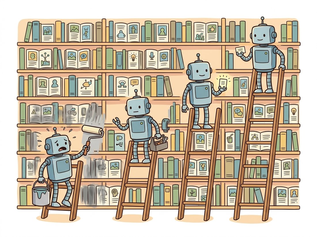
A Pretrained Generator Negotiating Its Next Lesson
Fine-tuning teaches a pretrained generator a new concept (a face, a product, a style) without retraining it from scratch, and the methods form a ladder from heaviest to lightest: full fine-tuning, then DreamBooth, then LoRA, then textual inversion, trading capacity for cost and forgetting risk. The central challenge is teaching the new thing without bulldozing everything the model already knows, and the methods differ mainly in how they protect the existing knowledge. This section walks the ladder, builds a LoRA fine-tune that runs on a single consumer GPU, and explains which method fits which job. It is the transfer-learning thread of Chapter 21 reaching its generative conclusion.
Prompting (Section 34.5) steers a model toward concepts it already knows. Fine-tuning teaches it concepts it does not. When you need your dog, this product, or a consistent character across a children's book (the studio from Section 34.3), no prompt suffices, because the concept is not in the training distribution. This section covers how to inject it. The transfer-learning principle is the one from Chapter 21: start from strong pretrained weights and adapt minimally, because adapting too much destroys the general capability you started from.
1. The Forgetting Problem and the Method Ladder Beginner
Naive fine-tuning has a signature failure: catastrophic forgetting. Train a billion-parameter generator on five photos of your dog and it will learn your dog and forget how to draw anything else, because the gradient from five images, applied to all parameters, overwrites the broad knowledge with the narrow. Every method on the ladder is a different answer to "how do I add the new concept without overwriting the old?" Table 34.6.1 lays out the ladder; the rest of the section explains each rung. The illustration below pictures the bargain: the heavier the change, the more of the existing library you risk smudging.
| Method | What changes | Storage | Forgetting risk | Best for |
|---|---|---|---|---|
| Full fine-tune | All weights | Full model (GBs) | High | A whole new domain, large data |
| DreamBooth | All weights + prior-preservation loss | Full model (GBs) | Medium (guarded) | A specific subject, high fidelity |
| LoRA | Small low-rank adapters | A few MB | Low | Subjects and styles, shareable |
| Textual inversion | One new embedding vector | A few KB | None (model frozen) | A concept describable as a "word" |
2. Textual Inversion: Learn One New Word Intermediate
The lightest method changes nothing in the model. Textual inversion freezes the entire generator and learns a single new embedding vector, a new "word" in the text encoder's vocabulary, that, when placed in a prompt, evokes the target concept. You introduce a pseudo-token like <my-dog>, initialize its embedding, and optimize only that vector so that "a photo of <my-dog>" reconstructs your training images under the frozen diffusion objective. Because the model is untouched, there is zero forgetting and the artifact is a few-kilobyte vector you can email. The cost is capacity: a single vector cannot capture fine appearance detail, so textual inversion is best for concepts that genuinely behave like a word (a recognizable style, a simple object) rather than a specific complex subject.
Mechanically it is the cleanest illustration of the whole chapter: it manipulates exactly the conditioning sequence of Section 34.1 and nothing else. The new word slots into the per-token embeddings, cross-attention (Section 34.2) routes it to the right spatial regions, and the frozen denoiser does the rest.
3. DreamBooth: Bind a Subject to a Rare Token Advanced
DreamBooth aims higher: faithful reproduction of a specific subject. It fine-tunes the whole model (or, in practice, combines with LoRA) to bind the subject to a rare token, "a photo of sks dog", where sks is chosen to have little prior meaning. The key idea that prevents forgetting is the prior-preservation loss. Alongside the few subject images, DreamBooth generates a batch of generic images from the model itself ("a photo of a dog") and includes them in training with their original captions. The model is thus simultaneously taught the new subject and reminded of the broad class, so it learns "sks dog is this particular dog" without collapsing the entire concept of "dog" onto your pet. The training objective is the standard diffusion loss plus the prior-preservation term:
$$ \mathcal{L} = \mathbb{E}\big[\|\epsilon - \epsilon_\theta(z_t, t, c_{\text{sks}})\|^2\big] + \lambda\,\mathbb{E}\big[\|\epsilon' - \epsilon_\theta(z'_{t'}, t', c_{\text{class}})\|^2\big], $$
where the first term learns the subject from your photos and the second, weighted by $\lambda$, preserves the class prior using the model's own generated class images. The prior-preservation term is the regularizer that guards the dictionary the epigraph worries about.
The famous sks token was supposed to be a meaningless string the model had no prior for, so that DreamBooth could fill it with your subject cleanly. There is a wrinkle: sks is also the name of a Soviet semi-automatic rifle, so it was never as empty as intended, and careful practitioners now pick genuinely rare tokens instead. The deeper point is the one that makes the whole method work: you are teaching the model a brand-new word, and the best new word is one the model has the fewest existing opinions about. The mnemonic for the ladder: freeze more, forget less.
4. LoRA: The Practical Default Intermediate
LoRA (Low-Rank Adaptation) is where most practitioners live, because it is cheap, shareable, and resistant to forgetting. The insight, borrowed from language models, is that the weight update needed to adapt a model to a new concept is low-rank: instead of learning a full update $\Delta W$ to a weight matrix $W \in \mathbb{R}^{d \times k}$, learn two small matrices $B \in \mathbb{R}^{d \times r}$ and $A \in \mathbb{R}^{r \times k}$ with rank $r \ll \min(d, k)$, and use $W + BA$ at inference. For a $1024 \times 1024$ matrix with $r = 8$, the two adapters hold $1024 \times 8$ entries in $B$ plus $8 \times 1024$ in $A$, so $2 \times 8192 = 16384$ trainable parameters replace the roughly one million in the full matrix, a 64-fold reduction. The base weights are frozen, so forgetting is minimal, and the adapter is a few megabytes you can publish and combine. LoRA is applied specifically to the cross-attention layers of Section 34.2, since that is where the text-to-image binding lives.
Figure 34.6.1 shows why LoRA is forgiving: the bulk of the model is frozen by construction, so the worst a bad LoRA can do is be ignored. The following script trains a LoRA on the cross-attention projections of an SD model, runnable on an 8 GB GPU.
import torch
from diffusers import StableDiffusionPipeline
from peft import LoraConfig, get_peft_model

pipe = StableDiffusionPipeline.from_pretrained(
    "stable-diffusion-v1-5/stable-diffusion-v1-5", torch_dtype=torch.float16).to("cuda")
unet = pipe.unet

# Inject rank-8 LoRA adapters into the cross-attention projection matrices only.
lora = LoraConfig(r=8, lora_alpha=16,
                  target_modules=["to_q", "to_k", "to_v", "to_out.0"])
unet = get_peft_model(unet, lora)
unet.print_trainable_parameters()
# e.g. trainable params: 797,184 || all params: 860,318,148 || trainable%: 0.09

opt = torch.optim.AdamW(
    [p for p in unet.parameters() if p.requires_grad], lr=1e-4)

for step, (latents, text_embeds) in enumerate(my_dataloader):  # your subject images
    noise = torch.randn_like(latents)
    t = torch.randint(0, 1000, (latents.size(0),), device="cuda")
    noisy = pipe.scheduler.add_noise(latents, noise, t)         # forward process
    pred = unet(noisy, t, encoder_hidden_states=text_embeds).sample
    loss = torch.nn.functional.mse_loss(pred, noise)            # noise-prediction loss
    loss.backward(); opt.step(); opt.zero_grad()

unet.save_pretrained("my-subject-lora") # a few MB, not the whole modelLoraConfig injects rank-8 adapters into the to_q, to_k, to_v, and to_out.0 cross-attention projections only, so just 0.09 percent of the parameters are trainable while the base U-Net stays frozen. The loop's mse_loss(pred, noise) is the same noise-prediction objective from Chapter 33, and save_pretrained writes a few-megabyte adapter rather than the gigabytes a full fine-tune would produce.
The print_trainable_parameters line is the whole pitch: under one percent of the model trains, which is why this fits on a consumer GPU in an afternoon and why the result is a shareable file rather than a model fork. Loading it back is one call, and adapters compose: a subject LoRA and a style LoRA can be applied together.
Every method that resists catastrophic forgetting does so by freezing the bulk of the model and confining the change to a small, isolated set of parameters: a single embedding (textual inversion), low-rank adapters (LoRA), or a regularized full update (DreamBooth's prior-preservation loss). The general capability lives in the frozen weights and cannot be overwritten by a few training images. This is the same principle as freezing a pretrained backbone in Chapter 21; generative fine-tuning simply makes the cost of forgetting more visible, because a forgotten generator produces visibly broken images.
You do not write the training loop above by hand for standard cases. The diffusers repository ships maintained training scripts for DreamBooth, textual inversion, and LoRA, and loading a trained LoRA into any pipeline is one call.
# Train via the official script (one shell command, abbreviated):
# accelerate launch train_dreambooth_lora.py \
#   --pretrained_model_name_or_path=stable-diffusion-v1-5/stable-diffusion-v1-5 \
#   --instance_data_dir=./my_dog --instance_prompt="a photo of sks dog" \
#   --rank=8 --output_dir=./my-dog-lora

from diffusers import StableDiffusionPipeline
import torch
pipe = StableDiffusionPipeline.from_pretrained(
    "stable-diffusion-v1-5/stable-diffusion-v1-5", torch_dtype=torch.float16).to("cuda")
pipe.load_lora_weights("./my-dog-lora")            # one line to attach the adapter
image = pipe("a photo of sks dog wearing sunglasses on the beach").images[0]train_dreambooth_lora.py script replaces the hand-written loop of Code Fragment 1, and load_lora_weights attaches the trained adapter to any compatible pipeline in one line. Multiple adapters can be loaded and weighted together, which is how community subject and style LoRAs are combined.Who: A consumer brand that needed hundreds of marketing images of its cartoon mascot in new scenes, all perfectly on-model (same proportions, colors, and face).
Situation: Prompting alone (Section 34.5) produced cousins of the mascot, never the mascot itself, because the exact character was not in the training distribution. They had about 40 clean reference images.
Problem: They first tried a full fine-tune, which nailed the mascot but forgot how to render the varied backgrounds and props the campaign needed: catastrophic forgetting from subsection 1, the whole-model update overwriting general scene knowledge with 40 mascot images.
Decision: They switched to a DreamBooth-plus-LoRA recipe: bind the mascot to a rare token with the prior-preservation loss of subsection 3 to keep "cartoon character" intact, and confine the update to rank-16 LoRA adapters (subsection 4) so the base model's scene knowledge stayed frozen. They captioned the 40 references descriptively, applying the DALL-E 3 caption lesson from Section 34.3.
Result: The mascot stayed on-model across hundreds of novel scenes, the model still rendered diverse backgrounds, and the deliverable was a 12 MB adapter the design team loaded into the stock pipeline. The full fine-tune's forgetting was solved by freezing plus prior preservation, not by more data.
Lesson: Match the rung to the job. A specific subject that must coexist with general capability calls for DreamBooth-plus-LoRA, not a full fine-tune; the freezing is what preserves the breadth, and descriptive captions on the references do as much work as the training algorithm.
The frontier in 2024 to 2026 is removing the per-subject training loop entirely. Encoder-based personalization methods (IP-Adapter, InstantID, PhotoMaker) take a reference image at inference time and inject its identity through a learned image encoder and extra cross-attention, with no fine-tuning per subject, the zero-shot end of the personalization ladder. DoRA (weight-decomposed LoRA, 2024) improves LoRA's capacity by separating magnitude and direction updates, narrowing the gap to full fine-tuning. On the controllability side, these adapters increasingly compose with the spatial-control methods of Chapter 35, so a single pipeline can fix identity, pose, and style at once. The arc is clear: from full fine-tuning (hours, gigabytes) to LoRA (minutes, megabytes) to tuning-free adapters (seconds, one reference image), the same efficiency descent that Chapter 28 traced for inference, now applied to customization.
The chapter ends where it began, at the assembly line. The Hands-On Lab below turns the three stations and three knobs of the opening key insight into a single program you build and run: it loads a generator, sweeps the prompt-engineering knobs of Section 34.5, swaps the model of Section 34.3, and finally bolts on a LoRA from this section so the same pipeline renders a concept the base model never saw.
Objective
Build a small, reproducible text-to-image studio: one script that loads a latent diffusion pipeline, generates from a prompt with fixed seeds, sweeps the guidance scale and a negative prompt to see the conditioning move, swaps in a second model behind the same interface, and attaches a LoRA adapter so the pipeline renders a new concept. The deliverable is a labeled contact sheet of generations that makes the chapter's three stations and three knobs visible at a glance.
What You'll Practice
- Treating the pipeline as the separable encode-generate-decode assembly line of Section 34.2 rather than one opaque box.
- Driving the prompt-engineering knobs of Section 34.5: guidance scale, negative prompts, and fixed seeds for reproducibility.
- Swapping the generator backbone behind one interface, the model-landscape lesson of Section 34.3.
- Attaching a LoRA adapter to customize the model on a single GPU (this section).
- Assembling the outputs into a labeled grid so each knob's effect is legible.
Setup
pip install diffusers transformers accelerate torch pillowA GPU with 8 GB or more makes each generation take seconds; on CPU it still runs but a single image may take a minute or more, so lower the step count and grid size. The base model, Stable Diffusion 1.5, downloads automatically on first run (about 4 GB). For the LoRA step you can use any small community LoRA from the Hugging Face Hub, or one you trained in Exercise 34.6.2.
Work the steps in order; each prints or saves a checkpoint so you can confirm progress before the next. A complete reference solution is folded at the end.
Step 1: Load the pipeline and expose its three stations
Load a latent diffusion pipeline and print the class of each station so the assembly line of Section 34.2 stops being abstract: a text encoder, a denoising U-Net, and a VAE decoder.
import torch
from diffusers import StableDiffusionPipeline

device = "cuda" if torch.cuda.is_available() else "cpu"
dtype = torch.float16 if device == "cuda" else torch.float32

pipe = StableDiffusionPipeline.from_pretrained(
    "runwayml/stable-diffusion-v1-5", torch_dtype=dtype
).to(device)
pipe.set_progress_bar_config(disable=True)

# TODO: print the class name of the three stations so the pipeline is concrete:
#       the text encoder (pipe.text_encoder), the generator (pipe.unet),
#       and the decoder (pipe.vae). Confirm they match Section 34.2's diagram.
Hint
print(type(pipe.text_encoder).__name__, type(pipe.unet).__name__, type(pipe.vae).__name__) reports CLIPTextModel, UNet2DConditionModel, and AutoencoderKL: the encode, generate, and decode stations the chapter opened with.
Step 2: Generate reproducibly with a fixed seed
A seed pins the starting noise so a generation is reproducible, the precondition for every comparison in Section 34.5. Write a helper that generates one image for a given prompt, guidance scale, negative prompt, and seed.
def generate(prompt, guidance=7.5, negative=None, seed=0, steps=30):
    gen = torch.Generator(device=device).manual_seed(seed)
    # TODO: call pipe(...) with prompt, negative_prompt=negative,
    #       guidance_scale=guidance, num_inference_steps=steps, generator=gen.
    #       Return result.images[0].
    ...

img = generate("a watercolor painting of a lighthouse at dawn", seed=0)
img.save("step2_base.png")
print("saved step2_base.png")
Hint
The body is return pipe(prompt, negative_prompt=negative, guidance_scale=guidance, num_inference_steps=steps, generator=gen).images[0]. Reusing the same seed with the same arguments reproduces the exact image, which is what lets the next step isolate one knob at a time.
Step 3: Sweep the guidance scale on one fixed seed
Guidance scale trades diversity for prompt fidelity (Section 34.5). Hold the seed and prompt fixed and vary only the guidance to see the fidelity-versus-artifact tradeoff directly.
prompt = "a watercolor painting of a lighthouse at dawn"
scales = [1.5, 4.0, 7.5, 12.0, 20.0]

# TODO: generate one image per scale with the SAME seed (e.g. 0), collect
#       them in a list `row`, and label each with its guidance value.
row = []
for g in scales:
    ...
print(f"collected {len(row)} images across guidance {scales}")
Hint
row = [generate(prompt, guidance=g, seed=0) for g in scales]. With the seed fixed, the only thing changing across the row is the guidance, so you can attribute every visible difference (washed-out at 1.5, oversaturated and artifacted at 20) to that single knob.
Step 4: Add a negative prompt and compare
A negative prompt steers the unconditional branch of classifier-free guidance away from unwanted content (Section 34.5). Generate a with-and-without pair on the same seed to isolate its effect.
neg = "blurry, low quality, extra fingers, watermark, text"

# TODO: generate two images on the same seed and guidance: one with
#       negative=None and one with negative=neg. Store them as a labeled pair.
pair = ...
print("generated the with/without negative-prompt pair")
Hint
pair = [("no negative", generate(prompt, seed=1, negative=None)), ("with negative", generate(prompt, seed=1, negative=neg))]. Keep every other argument identical so the only variable is the negative prompt.
Step 5: Swap the generator behind the same interface
The model landscape of Section 34.3 is the same template with different knobs. Load a second model into a pipeline with the identical generate contract and render the same prompt and seed through both.
from diffusers import DiffusionPipeline

pipe2 = DiffusionPipeline.from_pretrained(
    "stabilityai/sd-turbo", torch_dtype=dtype
).to(device)
pipe2.set_progress_bar_config(disable=True)

# TODO: render the same prompt and seed through pipe2. SD-Turbo is distilled
#       for very few steps, so use steps=1 and guidance=0.0. Note how the same
#       sentence yields a different look because the model knob changed.
gen2 = torch.Generator(device=device).manual_seed(0)
img_turbo = ...
img_turbo.save("step5_turbo.png")
Hint
img_turbo = pipe2(prompt, num_inference_steps=1, guidance_scale=0.0, generator=gen2).images[0]. SD-Turbo is a few-step distilled model (Chapter 33's consistency and distillation thread), so it ignores high guidance and finishes in one step; the comparison shows the generator knob changing the output, not the prompt.
Step 6: Attach a LoRA and render a new concept
Now bolt this section's customization onto the base pipeline. Load a LoRA adapter and generate with its trigger token so the same model renders a concept it did not know before.
# Use any SD-1.5-compatible LoRA on the Hub, or one you trained in Exercise 34.6.2.
# TODO: call pipe.load_lora_weights(REPO_OR_PATH) to attach the adapter, then
#       generate a prompt containing the LoRA's trigger token. Save the result.
...
img_lora = generate("a watercolor painting of a lighthouse, <trigger> style", seed=0)
img_lora.save("step6_lora.png")
pipe.unload_lora_weights()  # detach so later cells use the clean base model
print("saved step6_lora.png")
Hint
pipe.load_lora_weights("some-user/some-style-lora") attaches the rank-decomposed adapter in one line; load_lora_weights handles the weight injection of this section's subsection 4. Replace the placeholder trigger with the adapter's documented token. Call pipe.unload_lora_weights() when done so the base model is restored.
Step 7: Assemble a labeled contact sheet
Tie the runs together into one annotated grid so each knob's effect is visible side by side, the deliverable of the lab.
from PIL import Image, ImageDraw

def contact_sheet(labeled_images, cols=5, cell=256):
    rows = (len(labeled_images) + cols - 1) // cols
    sheet = Image.new("RGB", (cols * cell, rows * (cell + 22)), "white")
    draw = ImageDraw.Draw(sheet)
    for i, (label, im) in enumerate(labeled_images):
        x, y = (i % cols) * cell, (i // cols) * (cell + 22)
        sheet.paste(im.resize((cell, cell)), (x, y + 22))
        draw.text((x + 4, y + 4), label, fill="black")
    return sheet

# TODO: build a list of (label, image) tuples from the guidance sweep (Step 3),
#       the negative-prompt pair (Step 4), and the model swap (Step 5), then
#       call contact_sheet(...) and save it as studio_contact_sheet.png.
...
Hint
Collect tuples like [(f"g={g}", im) for g, im in zip(scales, row)] plus the Step 4 pair and a ("sd-turbo", img_turbo) entry, pass them to contact_sheet, and call .save("studio_contact_sheet.png"). The single image is the portfolio artifact that makes the three knobs legible.
Expected Output
Step 1 prints CLIPTextModel UNet2DConditionModel AutoencoderKL, the three stations named. The guidance sweep produces a five-image row where low guidance ($1.5$) looks washed out and only loosely matches the prompt, mid guidance ($7.5$) is the sweet spot, and high guidance ($20$) is oversaturated with contrast artifacts, the tradeoff of Section 34.5 made visual. The negative-prompt pair shows the cleaner image on the same seed once the unwanted terms are pushed out. The SD-Turbo swap renders a recognizable version of the same scene in a single step, visibly different in style because the model knob changed. The LoRA generation injects the adapter's concept or style into the lighthouse scene. The final studio_contact_sheet.png is a labeled grid that summarizes the whole study in one image: one prompt, three knobs, one assembly line.
Stretch Goals
- Add a seed grid: hold prompt and guidance fixed and vary only the seed across nine values, then render a 3-by-3 sheet showing the diversity a single prompt spans (Section 34.5).
- Swap the encoder station instead of the generator: load an SDXL pipeline (dual text encoder, Section 34.3) through the same
generatecontract and compare prompt following on a long compositional prompt, the encoder-ceiling argument of Section 34.1. - Compose two LoRAs (a subject and a style) into the pipeline with per-adapter weights, then sweep the weights and add the best result to the contact sheet, connecting to Exercise 34.6.2.
Complete Solution
import torch
from diffusers import StableDiffusionPipeline, DiffusionPipeline
from PIL import Image, ImageDraw

device = "cuda" if torch.cuda.is_available() else "cpu"
dtype = torch.float16 if device == "cuda" else torch.float32

# Step 1: load the pipeline and name the three stations.
pipe = StableDiffusionPipeline.from_pretrained(
    "runwayml/stable-diffusion-v1-5", torch_dtype=dtype
).to(device)
pipe.set_progress_bar_config(disable=True)
print(type(pipe.text_encoder).__name__,
      type(pipe.unet).__name__,
      type(pipe.vae).__name__)

# Step 2: a reproducible generation helper.
def generate(prompt, guidance=7.5, negative=None, seed=0, steps=30):
    gen = torch.Generator(device=device).manual_seed(seed)
    return pipe(prompt, negative_prompt=negative, guidance_scale=guidance,
                num_inference_steps=steps, generator=gen).images[0]

prompt = "a watercolor painting of a lighthouse at dawn"

# Step 3: guidance sweep on one fixed seed.
scales = [1.5, 4.0, 7.5, 12.0, 20.0]
row = [generate(prompt, guidance=g, seed=0) for g in scales]

# Step 4: negative-prompt comparison on a fixed seed.
neg = "blurry, low quality, extra fingers, watermark, text"
pair = [("no negative", generate(prompt, seed=1, negative=None)),
        ("with negative", generate(prompt, seed=1, negative=neg))]

# Step 5: swap the generator behind the same idea.
pipe2 = DiffusionPipeline.from_pretrained(
    "stabilityai/sd-turbo", torch_dtype=dtype
).to(device)
pipe2.set_progress_bar_config(disable=True)
gen2 = torch.Generator(device=device).manual_seed(0)
img_turbo = pipe2(prompt, num_inference_steps=1, guidance_scale=0.0,
                  generator=gen2).images[0]

# Step 6: attach a LoRA and render a new concept.
# Replace the repo id and trigger token with a real SD-1.5 LoRA.
try:
    pipe.load_lora_weights("ostris/watercolor_style_lora_sd15")
    img_lora = generate(prompt + ", watercolor style", seed=0)
    img_lora.save("step6_lora.png")
    pipe.unload_lora_weights()
except Exception as e:
    print("LoRA step skipped (supply a valid adapter):", e)

# Step 7: assemble the labeled contact sheet.
def contact_sheet(labeled_images, cols=5, cell=256):
    rows = (len(labeled_images) + cols - 1) // cols
    sheet = Image.new("RGB", (cols * cell, rows * (cell + 22)), "white")
    draw = ImageDraw.Draw(sheet)
    for i, (label, im) in enumerate(labeled_images):
        x, y = (i % cols) * cell, (i // cols) * (cell + 22)
        sheet.paste(im.resize((cell, cell)), (x, y + 22))
        draw.text((x + 4, y + 4), label, fill="black")
    return sheet

cells = [(f"g={g}", im) for g, im in zip(scales, row)]
cells += pair
cells += [("sd-turbo", img_turbo)]
contact_sheet(cells).save("studio_contact_sheet.png")
print("saved studio_contact_sheet.png")For each task, name the method on the ladder you would use and justify it from the forgetting-versus-capacity tradeoff of Table 34.6.1: (a) reproduce a specific person's face with high fidelity from 20 photos; (b) apply a consistent watercolor style to any prompt; (c) capture a simple recurring logo shape; (d) adapt a model to an entirely new domain (medical X-rays) with 50000 images. Then explain why DreamBooth needs a prior-preservation loss but textual inversion does not.
Using the official LoRA training script, train one LoRA on a subject (10 to 20 images of an object) and a second LoRA on a style (images sharing a consistent aesthetic). (a) Generate the subject in the style by loading both adapters into one pipeline and weighting them, and report how the result changes as you vary the two adapter weights. (b) Train the subject LoRA again at rank 4 and rank 32 and compare fidelity and overfitting (does rank 32 start memorizing backgrounds from the training images?). (c) Measure each adapter's file size and confirm it matches the parameter count from the rank.
Deliberately induce catastrophic forgetting: full-fine-tune a small SD model on 5 images of one subject with no prior-preservation loss and a high learning rate for many steps. (a) Track, every N steps, both the subject fidelity (does it look like the target?) and a "general capability" probe (generate "a red bus", "a mountain lake", "a bowl of soup") and describe how the general outputs degrade. (b) Re-run with the prior-preservation loss and with LoRA, and plot the forgetting curve for all three. (c) Relate the result to the freezing principle of the key-insight callout and to backbone freezing in Chapter 21.