Measuring Image Quality: FID, KID, Precision-Recall & CLIPScore

"My critic asked for a number. I do not have a number. I have a cloud of feature vectors and the strong opinion that it overlaps yours. Round that however you like."

An Inception Feature Extractor Refusing to Commit

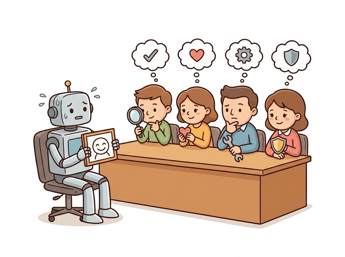
In Chapter 1 you measured restoration quality with PSNR and SSIM, and in Chapter 23 you measured detection with mAP. Both share a hidden assumption: there is a correct answer to compare against. A generator producing a face that has never existed breaks that assumption completely. There is no "true" image for the model to be close to, so per-image error is meaningless. What we can ask instead is a population question: does the set of images this model produces look, statistically, like the set of real images we trained on? That reframing, from per-sample error to distribution distance, is the conceptual leap of this section, and it is the place where the histogram and statistics thread from Chapter 2 grows up into a distance between entire image distributions. As the illustration below dramatizes, a shippable generator faces not one verdict but four separate audits at once.

1. From Pixels to Features: Why Inception Beginner

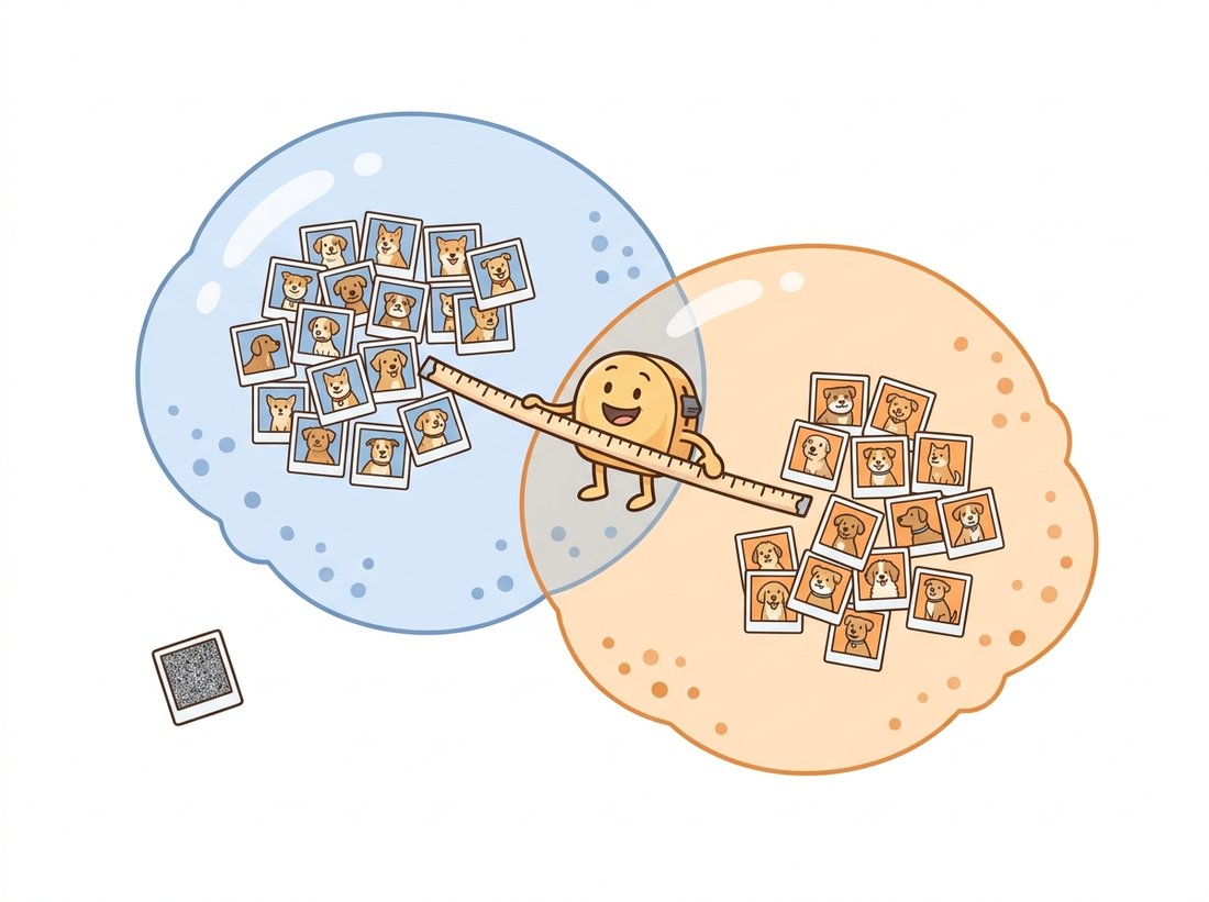
Comparing distributions of raw pixels is hopeless: two images of the same dog differ in millions of pixel values, and a metric in pixel space would call them wildly dissimilar. The fix, established by the Inception Score and then FID, is to compare distributions not in pixel space but in the feature space of a pretrained classifier. Run every image through a network trained on ImageNet, take the activations from a late layer (the 2048-dimensional pooling layer of Inception-v3 is the historical standard), and you get a vector that encodes semantic content (object identity, texture, layout) while discarding the pixel-level noise that does not matter. Two photos of dogs land near each other in this space; a photo and a blob of static land far apart. Those learned features are the same kind of representation you studied in Chapter 25; here we borrow them as a measuring stick rather than a backbone to fine-tune. With no single reference image to compare against, quality becomes the distance between two clouds of features, as the illustration below pictures.

The code below extracts pooled Inception-v3 features for a batch of images, the common preprocessing step underneath everything in this section. Figure 37.1.1 is exactly what this function feeds: the two feature clouds.

import torch
import torchvision.transforms as T
from torchvision.models import inception_v3, Inception_V3_Weights

device = "cuda" if torch.cuda.is_available() else "cpu"

# Load Inception-v3 and strip the classifier so forward() returns the
# 2048-dim pooled feature vector used by FID/KID/precision-recall.
weights = Inception_V3_Weights.IMAGENET1K_V1
net = inception_v3(weights=weights, aux_logits=True).to(device).eval()
net.fc = torch.nn.Identity()        # replace 1000-way head with a pass-through

prep = T.Compose([
    T.Resize(342), T.CenterCrop(299),          # Inception expects 299x299
    T.ToTensor(),
    T.Normalize([0.485, 0.456, 0.406], [0.229, 0.224, 0.225]),
])

@torch.no_grad()
def inception_features(images):
    """images: list of PIL.Image -> Tensor [N, 2048] of pooled features."""
    batch = torch.stack([prep(im.convert("RGB")) for im in images]).to(device)
    return net(batch).cpu()          # [N, 2048]

2. Frechet Inception Distance Intermediate

FID makes one modeling assumption: approximate each feature cloud as a single multivariate Gaussian, summarized by its mean vector and covariance matrix. Let the real features have mean $\mu_r$ and covariance $\Sigma_r$, and the generated features have mean $\mu_g$ and covariance $\Sigma_g$. The Frechet distance (also called the 2-Wasserstein distance) between two Gaussians has a closed form:

Here a covariance matrix $\Sigma$ records how each pair of feature dimensions varies together (its diagonal holds the per-dimension variances), and the trace $\operatorname{tr}(\cdot)$ is simply the sum of a matrix's diagonal entries. The first term penalizes a shift in the average feature (the generated images are, on average, a different kind of thing). The second term penalizes a mismatch in the spread and correlation structure (the generated images vary in the wrong ways). The matrix square root $(\Sigma_r \Sigma_g)^{1/2}$ is the only awkward piece; it is a real symmetric matrix square root, computed with an eigendecomposition or, in practice, the Schur-based scipy.linalg.sqrtm. Lower FID is better, and a perfect generator that exactly reproduces the real feature distribution scores zero. To see the two terms combine concretely, imagine the generated faces are shifted so their mean-feature vector sits a squared distance of $\lVert \mu_r - \mu_g \rVert_2^2 = 11.0$ from the real mean (the generator draws, on average, a slightly different kind of face), and the covariance-mismatch trace term works out to $7.4$ (the generated faces vary in subtly wrong ways): the two add to a final FID of $18.4$, the value the usage comment below prints. The implementation is a direct transcription of the formula.

import numpy as np
from scipy import linalg

def frechet_distance(feat_real, feat_gen):
    """feat_real, feat_gen: numpy arrays [N, D] of Inception features."""
    mu_r, mu_g = feat_real.mean(0), feat_gen.mean(0)
    # rowvar=False: each row is a sample, each column a feature dimension.
    sig_r = np.cov(feat_real, rowvar=False)
    sig_g = np.cov(feat_gen,  rowvar=False)

    diff = mu_r - mu_g
    covmean, _ = linalg.sqrtm(sig_r @ sig_g, disp=False)   # matrix square root
    if np.iscomplexobj(covmean):        # tiny imaginary parts from numerics
        covmean = covmean.real
    return float(diff @ diff + np.trace(sig_r + sig_g - 2 * covmean))

# Usage with the feature extractor from subsection 1:
# fr = inception_features(real_images).numpy()
# fg = inception_features(gen_images).numpy()
# print(f"FID = {frechet_distance(fr, fg):.2f}")   # e.g. FID = 18.43

Two properties matter in practice and bite people who ignore them. First, FID is biased: the estimate decreases as you use more samples, so an FID computed on 5,000 images is not comparable to one computed on 50,000. The bias falls roughly as $O(1/N)$ in the number of generated samples $N$, which is why two models must be compared at the identical sample count and why Chong and Forsyth (2020) proposed $\mathrm{FID}_\infty$, extrapolating a line fit of FID against $1/N$ to its $N\to\infty$ intercept to recover an unbiased value. The field standardized on 50,000 generated images against the full real set for exactly this reason. Second, FID is acutely sensitive to the image preprocessing pipeline. As the clean-fid paper (Parmar et al., 2022) demonstrated, using PIL bicubic resizing versus a different library's resizing can shift FID by several points, enough to flip the ranking of two models. Always report which pipeline you used, or use a standardized library.

from torchmetrics.image.fid import FrechetInceptionDistance

fid = FrechetInceptionDistance(feature=2048, normalize=True)
fid.update(real_batch, real=True)    # real_batch: [N,3,H,W] in [0,1]
fid.update(fake_batch, real=False)
print(fid.compute())                 # scalar tensor, e.g. tensor(18.43)

3. Kernel Inception Distance: Dropping the Gaussian Intermediate

FID's Gaussian assumption is a convenience, not a truth; feature distributions are rarely Gaussian. Kernel Inception Distance (KID) replaces it with a squared maximum mean discrepancy (MMD) using a polynomial kernel, which compares all the moments of the two distributions implicitly without assuming any particular shape. For features $x$ from the real set and $y$ from the generated set, the kernel is $k(x, y) = \left(\tfrac{1}{d}\, x^\top y + 1\right)^3$, where $d$ is the feature dimension, and the squared MMD is:

The decisive practical advantage over FID is that the standard estimator is unbiased: it does not systematically drift with sample count, so KID gives trustworthy numbers on a few thousand images where FID would still be moving. That makes KID the right choice when generating 50,000 samples is expensive, such as evaluating a slow video or 3D generator. The unbiased estimator drops the diagonal self-comparisons, which is the one subtlety in the code.

def poly_kernel(a, b):
    """Cubic polynomial kernel between feature sets a [m,D] and b [n,D]."""
    d = a.shape[1]
    return (a @ b.T / d + 1.0) ** 3         # [m, n] kernel matrix

def kid(feat_real, feat_gen):
    """Unbiased squared-MMD estimate (lower is better)."""
    m, n = len(feat_real), len(feat_gen)
    k_xx = poly_kernel(feat_real, feat_real)
    k_yy = poly_kernel(feat_gen,  feat_gen)
    k_xy = poly_kernel(feat_real, feat_gen)
    # Unbiased term removes the diagonal (self-similarity) before averaging.
    sum_xx = (k_xx.sum() - np.trace(k_xx)) / (m * (m - 1))
    sum_yy = (k_yy.sum() - np.trace(k_yy)) / (n * (n - 1))
    sum_xy = k_xy.sum() / (m * n)
    return float(sum_xx + sum_yy - 2 * sum_xy)

# Reported KID values are tiny; papers usually print KID x 1000.
# print(f"KID = {kid(fr, fg) * 1000:.3f}")    # e.g. KID = 1.742

4. Precision and Recall: Splitting Fidelity From Diversity Advanced

A single FID number hides a crucial ambiguity. A model can earn a mediocre FID two opposite ways: by producing a few flawless images that ignore most of the real distribution (high fidelity, low coverage, the classic GAN mode collapse from Chapter 32), or by producing a broad but blurry mess (low fidelity, high coverage, the classic VAE failure from Chapter 31). Improved precision and recall (Kynkaanniemi et al., 2019) disentangle these. The idea is geometric: estimate the real-data manifold (the region of feature space the real images actually occupy) as the union of small balls, one around each real feature, with radius equal to that point's distance to its $k$-th nearest real neighbor. Picturing it in two dimensions helps: drop a dot for every real feature, draw a small circle around each one sized to just reach its near neighbors, and the overlapping circles trace out the shape the real data covers; a generated point counts as "realistic" if it lands inside any of those circles. Then:

• Precision is the fraction of generated samples that fall inside the real manifold. It measures fidelity: are the generated images the kind of thing the real data contains?
• Recall is the fraction of real samples that fall inside the generated manifold. It measures coverage: does the generator reach all the variety the real data has?

Figure 37.1.2 makes the asymmetry visual: a mode-collapsed generator scores high precision and low recall, while an over-smoothed one does the reverse. The implementation builds the manifolds from k-nearest-neighbor radii and counts membership.

import torch

def knn_radii(feats, k=3):
    """Per-point radius = distance to its k-th nearest neighbor."""
    d = torch.cdist(feats, feats)                 # pairwise distances
    d.fill_diagonal_(float("inf"))                # ignore self
    return d.topk(k, largest=False).values[:, -1] # k-th smallest per row

def manifold_contains(manifold_feats, radii, query_feats):
    """Fraction of query points inside any ball of the manifold."""
    d = torch.cdist(query_feats, manifold_feats)  # [Q, M]
    inside = (d <= radii.unsqueeze(0)).any(dim=1) # within some real ball?
    return inside.float().mean().item()

def precision_recall(real, gen, k=3):
    r_real, r_gen = knn_radii(real, k), knn_radii(gen, k)
    precision = manifold_contains(real, r_real, gen)  # gen inside real
    recall    = manifold_contains(gen,  r_gen,  real) # real inside gen
    return precision, recall

# p, r = precision_recall(torch.tensor(fr), torch.tensor(fg))
# print(f"precision={p:.3f}  recall={r:.3f}")   # e.g. precision=0.78 recall=0.61

5. CLIPScore: Did the Image Match the Prompt? Intermediate

FID, KID, and precision-recall all measure whether generated images look like real images in general. For a text-to-image system from Chapter 34 that is only half the question; the other half is whether the image matches the specific prompt that asked for it. CLIPScore answers this by leaving the Inception family entirely and using the CLIP joint image-text embedding space you met in Chapter 25. Embed the image and the prompt with CLIP, and the cosine similarity between the two vectors, clamped at zero and scaled, is how well they agree:

The scaling constant $w = 2.5$ is a convention from the original paper that spreads scores into a readable range; it does not change rankings. Higher means better prompt alignment. The code uses the open_clip library to embed both modalities.

import torch, open_clip

model, _, preprocess = open_clip.create_model_and_transforms(
    "ViT-B-32", pretrained="laion2b_s34b_b79k")
tokenizer = open_clip.get_tokenizer("ViT-B-32")
model = model.eval()

@torch.no_grad()
def clip_score(image, prompt, w=2.5):
    """image: PIL.Image, prompt: str -> CLIPScore (higher = better match)."""
    img = preprocess(image).unsqueeze(0)
    txt = tokenizer([prompt])
    img_emb = model.encode_image(img)
    txt_emb = model.encode_text(txt)
    img_emb /= img_emb.norm(dim=-1, keepdim=True)   # L2-normalize for cosine
    txt_emb /= txt_emb.norm(dim=-1, keepdim=True)
    cos = (img_emb * txt_emb).sum(-1).clamp(min=0)
    return float(w * cos)

# clip_score(generated_image, "a red bicycle leaning on a brick wall")
# -> e.g. 0.81   (well-aligned prompts typically land around 0.7 to 0.9)

6. What These Metrics Miss Advanced

Every metric here is a proxy, and proxies can be gamed. FID rewards matching ImageNet-flavored statistics, so a model can lower FID by producing slightly oversaturated, texture-rich images that Inception likes, regardless of whether humans prefer them. CLIPScore rewards literal object presence, so it scores a list-of-objects image higher than a more artful interpretation. None of them sees a sixth finger, a melted-together pair of faces, or text that reads as gibberish, because those failures barely move pooled-feature statistics. The decisive evidence that the metrics are imperfect is that they disagree with humans, which is why human evaluation in Section 37.2 remains the gold standard rather than a luxury.