Human Evaluation & Preference Studies

"Three colleagues glanced at my output, said 'looks fine, I guess,' and I declared victory. A statistician later explained that I had measured the lunchtime mood of three people, not the quality of anything."

A Generative Model With a Premature Confidence Interval

Every automatic metric in Section 37.1 can be gamed, and for the questions people care about most (which image is more beautiful, which better follows a nuanced instruction, which hides a subtle artifact a person spots instantly) the only valid measurement is to ask people. The catch is that asking people badly is worse than not asking at all: a confident number from three distracted colleagues looks authoritative and means nothing. By the end of this section you will be able to design a preference study whose result actually means something and would replicate if someone else ran it. That is where the rigor of experimental design enters generative vision.

1. Why Humans, and Why It Is Hard Beginner

Three things make a generated image good in a way no Inception feature captures: aesthetic appeal, faithful adherence to a complex prompt, and the absence of the uncanny errors (extra fingers, garbled text, physically impossible lighting) that humans spot instantly and metrics shrug off. Asking people is the direct route, but human data is expensive, noisy, and full of biases. Raters anchor on the first option they see, prefer brighter or more saturated images regardless of the question asked, get tired and lazy halfway through a session, and disagree with each other in ways that are sometimes real signal and sometimes pure noise. A study that does not control for these produces a number that looks authoritative and means nothing. The defense is design: control what each rater sees, ask one precise question, and collect enough independent judgments that the noise averages out.

2. The Two-Alternative Forced-Choice Protocol Beginner

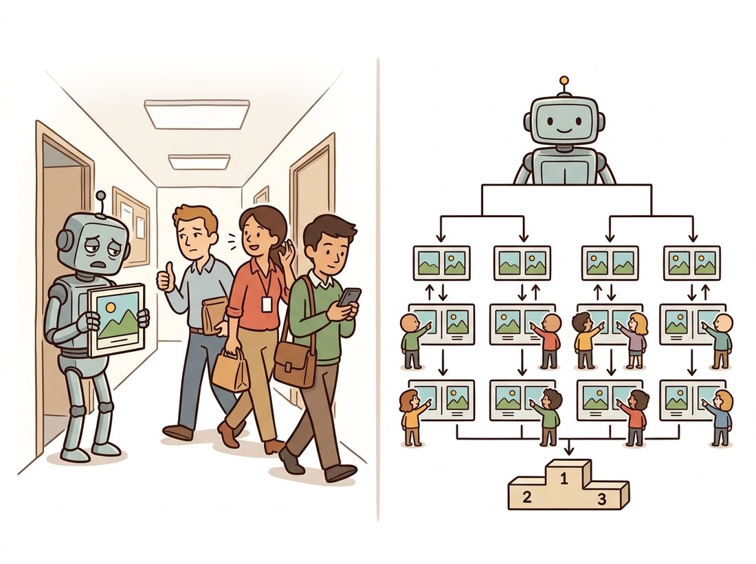
The workhorse design is two-alternative forced choice (2AFC): show a rater the same prompt rendered by two different models, side by side, in randomized left-right order, and force a choice of which is better on one stated axis (overall quality, or prompt alignment, or photorealism, pick one per study). Randomizing position defeats the left-side bias; forcing a choice (no "they are equal" escape hatch, or a separate explicit tie option counted carefully) yields cleaner statistics; asking one axis at a time stops raters from silently averaging incompatible criteria. Figure 37.2.1 lays out the design and the data it produces.

The two design parameters that decide whether the study has any power are the number of distinct prompts (item diversity) and the number of independent judgments per pair (statistical depth). Too few prompts and you measure quality on a handful of cherry-picked scenes; too few judgments and your win rate is dominated by sampling noise. A back-of-the-envelope power calculation tells you how many comparisons you need to detect a given win-rate gap.

import math
from scipy import stats

def comparisons_needed(p_win, alpha=0.05, power=0.80):
    """How many 2AFC judgments to distinguish win rate p_win from 0.5.

    p_win: the true win rate you want to be able to detect (e.g. 0.55).
    Returns the approximate number of independent comparisons required.
    """
    z_a = stats.norm.ppf(1 - alpha / 2)     # two-sided significance
    z_b = stats.norm.ppf(power)             # desired power
    effect = abs(p_win - 0.5)
    var = p_win * (1 - p_win)
    n = ((z_a + z_b) ** 2 * var) / (effect ** 2)
    return math.ceil(n)

print(comparisons_needed(0.55))   # detect a 55/45 split -> 778
print(comparisons_needed(0.60))   # detect a 60/40 split -> 188

3. Inter-Rater Agreement: Is the Signal Real? Intermediate

Suppose your raters split 60-40 in favor of Model A. Before you trust that, ask whether the raters agree with each other. If different raters pick essentially at random and the 60-40 split is an aggregation artifact, the result is meaningless. Inter-rater reliability quantifies agreement beyond what chance alone would produce. For two raters on categorical choices, Cohen's kappa is standard; for many raters and missing data, Krippendorff's alpha is the general tool. Both correct for chance agreement: a value of 1 is perfect agreement, 0 is chance-level, and negative values mean systematic disagreement. The code computes Cohen's kappa for a pair of raters.

def cohens_kappa(rater_a, rater_b):
    """Chance-corrected agreement for two raters on the same items.

    rater_a, rater_b: lists of categorical choices ("A" or "B") on the
    same set of comparison trials, in the same order.
    """
    n = len(rater_a)
    cats = set(rater_a) | set(rater_b)
    observed = sum(x == y for x, y in zip(rater_a, rater_b)) / n
    # Expected agreement if both rated independently at their own base rates.
    expected = sum(
        (rater_a.count(c) / n) * (rater_b.count(c) / n) for c in cats
    )
    return (observed - expected) / (1 - expected)

a = ["A", "A", "B", "A", "B", "B", "A", "B"]
b = ["A", "B", "B", "A", "B", "A", "A", "B"]
print(f"kappa = {cohens_kappa(a, b):.3f}")   # kappa = 0.500 (moderate)

Low agreement is not always a failure of the raters; sometimes it tells you the question is genuinely ambiguous or that the two models are close enough that the difference is below human perceptual resolution. A study that reports a win rate without an agreement statistic is incomplete, because the reader cannot tell whether the preference is a real signal or rater noise dressed up as one.

4. From Pairwise Wins to a Ranking: Bradley-Terry and Elo Intermediate

When you compare more than two models, you do not run every pair to convergence; you collect a sparse, irregular set of pairwise outcomes and need a single ranking out of them. The Bradley-Terry model assigns each model a latent strength score $s_i$ and predicts the probability that model $i$ beats model $j$ as a logistic function of the score difference:

Here $\sigma$ is the same logistic sigmoid you met training classifiers, squashing the score gap $s_i - s_j$ into a win probability between 0 and 1; equal strengths give the gap zero and the probability one-half, exactly the coin flip you would expect between evenly matched models. Fitting the scores by maximum likelihood to the observed win-loss matrix gives a principled global ranking even from sparse comparisons.

The Elo rating familiar from chess is an online approximation of the same model that updates scores incrementally after each match: it nudges the winner's score up and the loser's down by an amount proportional to how surprising the result was (beating a much stronger opponent moves the needle far more than beating a weaker one), which is exactly the gradient step of the Bradley-Terry log-likelihood taken one match at a time. That online form is what an arena needs, because votes arrive as a never-ending stream and new models keep joining: you want each battle to update the ranking immediately without re-fitting the entire history, which is why public "arena" leaderboards (where users vote on anonymized model outputs in a stream of head-to-head battles) report Elo or Bradley-Terry scores. The function below fits Bradley-Terry strengths from a win matrix by gradient ascent.

import numpy as np

def bradley_terry(win_matrix, iters=200, lr=0.1):
    """Fit latent strengths from a win matrix W[i,j] = times i beat j."""
    n = win_matrix.shape[0]
    s = np.zeros(n)                          # init all strengths equal
    for _ in range(iters):
        grad = np.zeros(n)
        for i in range(n):
            for j in range(n):
                if i == j:
                    continue
                games = win_matrix[i, j] + win_matrix[j, i]
                if games == 0:
                    continue
                p_ij = 1 / (1 + np.exp(-(s[i] - s[j])))    # predicted P(i beats j)
                grad[i] += win_matrix[i, j] - games * p_ij # observed minus expected
        s += lr * grad
        s -= s.mean()                        # fix the free additive constant
    return s

# Three models; rows beat columns this many times.
W = np.array([[0, 70, 85],
              [30, 0, 60],
              [15, 40, 0]], dtype=float)
print(np.round(bradley_terry(W), 3))   # e.g. [ 0.74  0.03 -0.77 ]  -> model 0 strongest

5. From Preference Data to Trained Models Advanced

Once you can collect human preferences at scale, they stop being only an evaluation tool and become a training signal. A reward model is a network trained on the preference pairs to predict which of two images a human would choose; structurally it is a Bradley-Terry head on top of an image (and often text) encoder, optimizing exactly the logistic objective of subsection 4 but with learned features instead of fixed per-model scores. Once trained, the reward model scores any new image, so it serves both as a fast automatic stand-in for human judgment (this is precisely what ImageReward and PickScore from Section 37.1 are) and as the optimization target for preference tuning, where a generator is fine-tuned to produce images the reward model rates highly. This mirrors the reinforcement-learning-from-human-feedback (RLHF) recipe that aligned large language models, transplanted to diffusion via methods like Diffusion-DPO (Direct Preference Optimization applied to a diffusion model). The thread connects to the transfer-learning recipes of Chapter 21: the reward model is a fine-tuned foundation encoder of the kind built in Chapter 25, and the preference-tuned generator is the same diffusion backbone from Chapter 33 nudged by a new loss. Figure 37.2.2 traces this closed loop: the same forced-choice judgments that evaluated the generator come back around to train it.