Image Formation: Optics, Sensors & the ISP Pipeline

"People say I have a great eye. Technically I have twelve million of them, and each one counts photons for a living."

A Slightly Overexposed Image Sensor

In Chapter 0 we treated the image as a given: a NumPy array that appears when you call cv2.imread. This section asks the question that chapter deliberately postponed: where does that array come from? The answer is a journey in three legs. Optics focuses light from the scene onto a plane. A sensor converts that light into numbers, one photosite at a time, with physics-imposed noise. And an ISP transforms the sensor's raw, greenish, linear measurements into the cheerful JPEG your code eventually loads. Each leg leaves fingerprints in the data that you will keep encountering for the rest of this book.

1. From Scene to Sensor: The Optics Beginner

The simplest camera is a box with a hole. The pinhole camera maps each scene point onto the image plane along a straight ray, producing a perfectly sharp but extremely dim image, because almost no light fits through the hole. Real cameras replace the pinhole with a lens, which gathers a wide cone of light from each scene point and refocuses it back to (approximately) a single image point. The price of that brightness is the focusing constraint captured by the thin lens equation:

where $f$ is the focal length, $z_o$ is the distance from the lens to the object, and $z_i$ is the distance from the lens to the image plane. Only objects at one particular $z_o$ are perfectly in focus for a given $z_i$; everything else is blurred into a small disk (the circle of confusion). The range of depths that look acceptably sharp is the depth of field.

Two numbers on a lens barrel summarize most of its optical behavior. The focal length $f$ sets the field of view: short focal lengths see wide, long focal lengths see narrow and magnified. The f-number $N = f / D$, where $D$ is the aperture diameter, sets how much light gets in. Small $N$ (a wide aperture like f/1.8) means more light and shallower depth of field; large $N$ (f/11) means less light and deeper focus. There is a hard physical floor here: even a perfect lens blurs a point into a diffraction pattern whose central disk has diameter roughly $2.44 \, \lambda N$ for wavelength $\lambda$. At f/8 and green light ($\lambda \approx 550$ nm) that disk is about 10.7 µm wide, several times larger than the pixels on a modern phone sensor. Past a certain point, more megapixels measure the blur more precisely rather than seeing more detail, a theme we quantify in Section 1.3.

2. The Sensor: Counting Photons Intermediate

At the image plane sits a CMOS sensor: a grid of millions of photosites, each a tiny silicon well that converts incoming photons into electrons via the photoelectric effect. During the exposure time, each well accumulates charge roughly proportional to the light hitting it. At readout, the charge is amplified (the gain is what your camera calls ISO) and digitized by an analog-to-digital converter into a 10, 12, or 14 bit integer. Three properties of this process matter enormously for everything downstream.

First, the response is linear. Twice the photons means twice the electrons means twice the digital number, right up until the well fills. That fullness threshold is the full well capacity, and hitting it is what clipping means physically: the well simply cannot hold more charge, and every brighter scene value maps to the same maximum number. Clipped highlights are unrecoverable, a fact that drives the dynamic range engineering of Section 1.3.

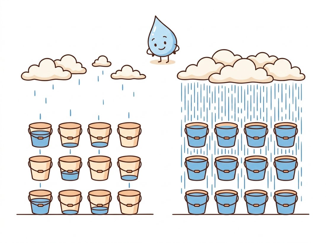
Second, light itself is noisy. Photons arrive randomly, following Poisson statistics: a pixel that should receive $n$ photons on average actually receives $n \pm \sqrt{n}$. The signal-to-noise ratio of this photon shot noise is therefore

which explains, in one line, why low-light images are grainy: fewer photons per pixel means lower $\sqrt{n}$, and no sensor design can change the statistics of the light itself. The simulation below makes this concrete with nothing but a Poisson random generator.

import numpy as np

rng = np.random.default_rng(seed=7)

# A perfectly uniform gray patch imaged at four light levels.
# The ONLY noise source here is the Poisson arrival of photons.
for n_photons in [10, 100, 1_000, 10_000]:
    ideal = np.full((256, 256), n_photons, dtype=np.float64)
    captured = rng.poisson(ideal)            # photon shot noise
    snr = captured.mean() / captured.std()
    print(f"{n_photons:>6} photons/pixel -> SNR = {snr:6.1f}"
          f"  (theory sqrt(n) = {np.sqrt(n_photons):6.1f})")

    10 photons/pixel -> SNR =    3.2  (theory sqrt(n) =    3.2)
   100 photons/pixel -> SNR =   10.0  (theory sqrt(n) =   10.0)
  1000 photons/pixel -> SNR =   31.6  (theory sqrt(n) =   31.6)
 10000 photons/pixel -> SNR =  100.0  (theory sqrt(n) =  100.0)

Third, the electronics add their own noise on top: read noise from the amplifier, dark current from thermally generated electrons, and fixed-pattern noise from manufacturing variations between photosites. In bright light, shot noise dominates; in deep shadow, read noise takes over. This is why denoising algorithms, from the classical filters of Chapter 7 to learned methods, benefit from knowing the noise model: the variance of a raw pixel is approximately a linear function of its brightness, not a constant.

3. The Color Problem: One Sensor, Three Channels Intermediate

Silicon photosites count photons; they do not perceive color. To capture color with a single sensor, manufacturers overlay a color filter array (CFA), almost always the Bayer pattern: a repeating 2×2 tile with one red filter, one blue filter, and two green filters (green is doubled because human luminance sensitivity peaks in green). The consequence is startling when you first meet it: a 12 megapixel camera measures only 12 million color samples in total, one per pixel, not 36 million. At every pixel, two of the three RGB values you find in your array were never measured. They were invented.

The inventing step is demosaicing: interpolating each missing channel from its neighbors. Simple bilinear interpolation works on smooth regions but produces colored fringing ("zippering") near edges, so production demosaicers use edge-aware methods. The code below builds a Bayer mosaic from a known RGB image and reconstructs it, so you can measure exactly what demosaicing gets wrong and where.

import cv2
import numpy as np

# Synthetic test scene: smooth ramps plus stripes (no input files needed).
h, w = 256, 384
yy, xx = np.mgrid[0:h, 0:w].astype(np.float32)
rgb = np.dstack([
    255 * xx / (w - 1),                 # red ramps left to right
    255 * yy / (h - 1),                 # green ramps top to bottom
    128 + 64 * np.sin(xx / 6.0),        # blue stripes add sharp detail
]).astype(np.uint8)

# 1. Sample through an RGGB color filter array: ONE value per photosite.
mosaic = np.zeros((h, w), dtype=np.uint8)
mosaic[0::2, 0::2] = rgb[0::2, 0::2, 0]   # R photosites
mosaic[0::2, 1::2] = rgb[0::2, 1::2, 1]   # G photosites (even rows)
mosaic[1::2, 0::2] = rgb[1::2, 0::2, 1]   # G photosites (odd rows)
mosaic[1::2, 1::2] = rgb[1::2, 1::2, 2]   # B photosites

# 2. Demosaic: interpolate the two missing channels at every pixel.
#    OpenCV names Bayer patterns by the 2x2 tile starting at pixel (1, 1),
#    so an RGGB mosaic uses the constant COLOR_BayerBG2RGB.
demosaiced = cv2.cvtColor(mosaic, cv2.COLOR_BayerBG2RGB)

err = np.abs(demosaiced.astype(np.int16) - rgb.astype(np.int16))
print("mean abs reconstruction error:", round(float(err.mean()), 2))
print("99th percentile error:", int(np.percentile(err, 99)))

4. The ISP Pipeline: From Raw Counts to a Viewable Image Intermediate

Between the sensor's raw mosaic and the file you load lies the image signal processor, a dedicated chip (or firmware block) that executes a fixed sequence of transformations at billions of pixels per second. Figure 1.1.1 traces the canonical stages. Real ISPs vary the order and fuse stages, but the logical flow is remarkably stable across vendors.

Walking through the dashed box in Figure 1.1.1: black level subtraction removes the sensor's electronic pedestal; white balance multiplies the R and B channels by gains so that the scene's illuminant (sunlight, tungsten, LED) renders neutrals as neutral; demosaicing fills in the missing color samples as in Code 1.1.2; the color correction matrix maps the sensor's idiosyncratic spectral sensitivities into a standard color space; the tone curve and gamma encoding compress the sensor's linear 12 to 14 bit range into perceptually spaced 8 bit values (we will treat gamma carefully when we meet point operations in Chapter 2); and finally denoising plus sharpening trades texture for cleanliness in a way each vendor tunes to taste. Every one of these stages destroys information: clipping in white balance, interpolation error in demosaicing, quantization in tone mapping, and texture loss in denoising are all permanent.

import rawpy

with rawpy.imread("photo.dng") as raw:
    rgb = raw.postprocess(use_camera_wb=True,   # apply as-shot white balance
                          output_bps=16,        # keep 16 bit precision
                          no_auto_bright=True)  # no surprise exposure changes
print(rgb.shape, rgb.dtype)   # e.g. (4024, 6048, 3) uint16

5. Why Vision Engineers Should Care Beginner

It is tempting to shrug: the camera produces an image, the model consumes it, why study the plumbing? Three practical reasons. First, ISPs are tuned for human viewing, not for machine consumption; aggressive sharpening creates halo edges that confuse gradient-based methods, and denoising erases the fine texture that classifiers use to tell surfaces apart. Second, the pipeline is not fixed across devices: the same scene shot on two phones yields measurably different arrays, which is a silent domain shift for any deployed model, and a key reason production teams covered in Chapter 28 care about controlling the capture stack on edge devices. Third, several classic "image processing" operations (white balance, gamma, denoising) are things the ISP already did once; doing them again naively compounds errors.

There is also an opportunity hiding here. Because the RAW mosaic is linear in light, it supports physically meaningful arithmetic: averaging RAW frames genuinely averages photons, and noise behaves predictably. Computational photography exploits this constantly, and a growing line of research feeds RAW data directly to neural networks, skipping the ISP's human-oriented choices altogether.

With formation physics in hand, the next question is mathematical: what does it mean to chop a continuous optical image into a finite grid of finite-precision numbers? That is sampling and quantization, the subject of Section 1.2.