Classical Denoising: From Gaussian to Non-Local Means

"Why should I average my neighbors just because they live next door? Somewhere across this image are patches that actually understand me."

A Non-Local Means Filter With High Standards

Section 7.1 built the damage: we can now synthesize noise with known statistics and score any attempted cure with the PSNR and SSIM metrics from Chapter 1. This section attempts the cure itself. We start from the humble filters of Chapter 3, reread them as denoisers, and then make the conceptual leap that defined classical denoising's final and best decade: the realization that a pixel's most trustworthy relatives usually do not live next door.

1. Averaging and Its Discontents Beginner

All denoising rests on one statistical fact. If you average $N$ independent measurements of the same underlying value, each corrupted by noise of standard deviation $\sigma$, the average has noise $\sigma / \sqrt{N}$. Average a hundred honest copies of a pixel and the noise drops tenfold. The entire difficulty of denoising hides inside the phrase "of the same underlying value": the clean image is exactly what we do not have, so we never know for certain which pixels share a value. Every algorithm in this section is a strategy for guessing.

Guess too generously and you average pixels that do not belong together: an edge pixel gets blended with the other side of the edge, and noise reduction becomes blur. Guess too cautiously and you average too few samples, leaving noise behind. This is the denoiser's version of the bias-variance tradeoff: aggressive averaging trades variance (noise) for bias (lost structure). The history of classical denoising is the history of finding more pixels to average without inviting the wrong ones, and you can read the whole section as a progression of increasingly clever invitation lists.

2. The Local Family, Reread as Denoisers Beginner

Chapter 3 introduced the Gaussian, median, and bilateral filters as general smoothing tools. Viewed as denoisers, each is an invitation policy. The Gaussian filter invites every pixel within a spatial radius, weighted by distance: its prior says images are smooth everywhere, which is false at every edge, and the result is the familiar tradeoff of clean flat regions bought with smeared boundaries. The median filter invites the same neighbors but takes a vote instead of an average, which makes it nearly immune to the impulse noise of Table 7.1.1: a dead pixel is an outlier, and medians ignore outliers. The bilateral filter adds a second gate: a neighbor is invited only if it is both spatially close and tonally similar, so averaging stops at edges. Code 7.2.1 runs all three against the same Gaussian-noised test image so we have concrete numbers to argue about.

import numpy as np
from skimage import data, img_as_float
from skimage.filters import gaussian, median
from skimage.morphology import disk
from skimage.restoration import denoise_bilateral
from skimage.metrics import peak_signal_noise_ratio as psnr

rng = np.random.default_rng(seed=7)
clean = img_as_float(data.camera())                    # 512x512 grayscale
noisy = np.clip(clean + rng.normal(0, 0.10, clean.shape), 0, 1)

results = {
    'noisy':     noisy,
    'gaussian':  gaussian(noisy, sigma=1.2),
    'median':    median(noisy, footprint=disk(2)),
    'bilateral': denoise_bilateral(noisy, sigma_color=0.15, sigma_spatial=3),
}
for name, img in results.items():
    print(f"{name:9s} PSNR = {psnr(clean, img):.1f} dB")

noisy     PSNR = 20.2 dB
gaussian  PSNR = 26.5 dB
median    PSNR = 25.6 dB
bilateral PSNR = 26.9 dB

The bilateral filter's waxiness is worth understanding because it motivates everything that follows. The tonal gate works well at high-contrast edges, where "similar intensity" reliably means "same side of the edge." But in low-contrast texture, noise itself decides who looks similar: the filter averages pixels whose intensities happen to match by chance, producing the smooth, plasticky patches that photographers call the watercolor effect. The deeper problem is that a single noisy pixel value is a terrible identity card. Two pixels from the same structure can differ wildly because of noise; two pixels from different structures can match by accident. We need a richer description of who a pixel is.

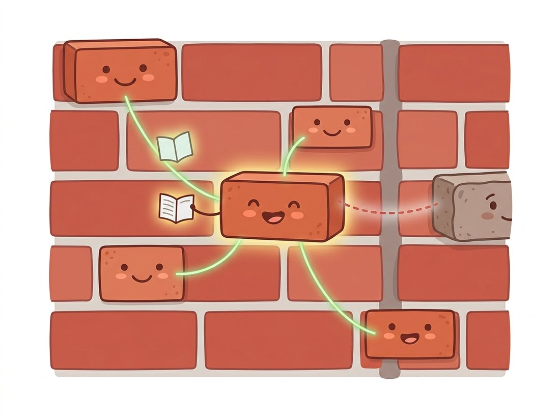
3. Non-Local Means: Averaging by Resemblance Intermediate

The 2005 insight of Buades, Coll, and Morel reads obvious in hindsight, as the best insights do. Natural images are massively self-similar: a brick wall contains hundreds of nearly identical bricks, a face has two matching eyebrows and acres of similar skin, a sky repeats itself almost everywhere. Each repetition is an independent noisy measurement of nearly the same content. So instead of identifying a pixel by its single noisy value, identify it by the small patch around it, and average it with every pixel in the image whose surrounding patch looks alike, regardless of where that pixel lives. The estimate for pixel $p$ becomes

where $P(p)$ is the patch of pixels centered on $p$, $Z(p) = \sum_q w(p,q)$ normalizes the weights, and $h$ controls how strict the resemblance test is. Patches that match closely get weight near one; patches that differ get exponentially suppressed. Figure 7.2.1 contrasts this with the local policy of Section 2: the bilateral filter asks "who is nearby and similar in value," while non-local means (NLM) asks "who, anywhere, is living the same life."

Code 7.2.2 is a deliberately naive implementation, four nested loops and no tricks, because the algorithm fits in fifteen readable lines and reading it teaches more than any description. Run it on a small crop; the full image would take minutes, which is itself a lesson about why the optimized library versions exist.

def nlm_gray(img, patch=7, window=8, h=0.12):
    """Educational non-local means for float grayscale images.
    Searches a (2*window+1)^2 neighborhood; O(N * window^2 * patch^2)."""
    half = patch // 2
    pad = half + window
    p = np.pad(img, pad, mode='reflect')
    out = np.empty_like(img)
    for i in range(img.shape[0]):
        for j in range(img.shape[1]):
            ci, cj = i + pad, j + pad
            ref = p[ci-half:ci+half+1, cj-half:cj+half+1]
            wsum, acc = 0.0, 0.0
            for di in range(-window, window + 1):
                for dj in range(-window, window + 1):
                    cand = p[ci+di-half:ci+di+half+1,
                             cj+dj-half:cj+dj+half+1]
                    d2 = np.mean((ref - cand) ** 2)     # patch distance
                    w = np.exp(-d2 / h ** 2)            # resemblance weight
                    wsum += w
                    acc  += w * p[ci + di, cj + dj]
            out[i, j] = acc / wsum
    return out

crop, ncrop = clean[120:184, 200:264], noisy[120:184, 200:264]
restored = nlm_gray(ncrop)
print(f"noisy crop PSNR = {psnr(crop, ncrop):.1f} dB, "
      f"NLM crop PSNR = {psnr(crop, restored):.1f} dB")

Two parameters do the steering. The patch size (7x7 is the classic default) sets how much context defines a pixel's identity: too small and noise corrupts the identity card, too large and rare structures find no matches. The bandwidth $h$ sets the strictness of the resemblance test and should scale with the noise level: a common refinement subtracts the expected noise contribution from the patch distance before weighting, $w = \exp(-\max(d^2 - 2\sigma^2, 0)/h^2)$, so that two identical patches corrupted by noise still count as identical. The exercises ask you to implement that version, and feeding it the $\sigma$ estimated by Code 7.1.3 closes the loop with the previous section.

import cv2
from skimage.restoration import denoise_nl_means, estimate_sigma

# OpenCV: uint8 in, strength h in 8-bit gray levels (about the noise sigma)
den_cv = cv2.fastNlMeansDenoising((noisy * 255).astype(np.uint8), None,
                                  h=25, templateWindowSize=7,
                                  searchWindowSize=21)

# scikit-image: float in, noise-aware weighting via sigma=
sigma_est = estimate_sigma(noisy)
den_sk = denoise_nl_means(noisy, h=0.8 * sigma_est, sigma=sigma_est,
                          patch_size=7, patch_distance=11, fast_mode=True)

4. BM3D: Self-Similarity Meets Sparsity Advanced

Non-local means uses similar patches timidly: it only averages their center pixels. BM3D (block-matching and 3D filtering, Dabov et al. 2007) commits fully. It groups similar patches into a 3D stack, applies a 3D transform to the whole stack (a 2D DCT or wavelet across each patch, plus a 1D transform along the stack), and then denoises all the patches jointly by shrinking small transform coefficients toward zero. The logic combines both great classical priors at once. Self-similarity says the stacked patches are nearly identical, so the 1D transform along the stack compresses them into a few strong coefficients. Transform-domain sparsity, the idea behind the wavelet shrinkage you met in Chapter 4, says clean structure concentrates in few large coefficients while noise spreads evenly across all of them. Kill the small coefficients and you kill mostly noise; the patches then "collaborate," because structure shared across the group survives shrinkage even where any single patch is too noisy to reveal it.

The full algorithm runs this pipeline twice: a first pass with hard thresholding produces a rough estimate, and a second pass uses that estimate to build Wiener shrinkage weights (the same Wiener logic that Section 7.3 derives for deblurring) for a refined result. Patches overlap, so each pixel receives many estimates that are averaged with weights. None of this is pleasant to implement, and unlike NLM there is no fifteen-line educational version worth your time; the reference implementation from the original authors is the sensible route, shown in Code 7.2.4.

import bm3d                      # pip install bm3d  (Tampere reference impl.)

den_bm3d = bm3d.bm3d(noisy, sigma_psd=0.10,
                     stage_arg=bm3d.BM3DStages.ALL_STAGES)
print(f"BM3D PSNR = {psnr(clean, den_bm3d):.1f} dB")

BM3D PSNR = 29.4 dB

From 2007 until deep denoisers matured in the late 2010s, BM3D was the number to beat, and it aged remarkably well: it needs no training data, adapts to any noise level through a single parameter, and remains the standard "classical baseline" row in every denoising paper's results table. When a learned method beats BM3D by half a decibel, that half decibel is the headline.

5. The Bake-Off, and What the Numbers Hide Intermediate

Code 7.2.5 races the contenders on equal terms, measuring both quality and time, because in production the second number often decides. The ranking it produces is the canonical one: quality rises in the order Gaussian, median, bilateral, NLM, BM3D, and runtime rises in nearly the same order. You pay for trust.

import time

def bench(name, fn):
    t0 = time.perf_counter()
    out = fn()
    ms = (time.perf_counter() - t0) * 1000
    print(f"{name:10s} {psnr(clean, out):5.1f} dB   {ms:8.0f} ms")

bench('gaussian',  lambda: gaussian(noisy, sigma=1.2))
bench('bilateral', lambda: denoise_bilateral(noisy, sigma_color=0.15,
                                             sigma_spatial=3))
bench('nl-means',  lambda: denoise_nl_means(noisy, h=0.8 * sigma_est,
                                            sigma=sigma_est, patch_size=7,
                                            patch_distance=11, fast_mode=True))
bench('bm3d',      lambda: bm3d.bm3d(noisy, sigma_psd=0.10))

gaussian    26.5 dB         6 ms
bilateral   26.9 dB       310 ms
nl-means    28.3 dB       900 ms
bm3d        29.4 dB      4600 ms

Now the caveats, because this tidy benchmark hides three traps. First, everything above assumes additive Gaussian noise of known strength; on the Poisson-dominated low-light images of Section 7.1, run the Anscombe sandwich around any of these methods or the dark regions will be under-denoised. Second, PSNR rewards smoothness, as Section 7.1 warned: the bilateral filter's waxy patches score better than they look, and BM3D's occasional low-contrast artifacts (ghostly repeated structure in flat areas, the price of aggressive patch grouping) score worse than they look. Always look. Third, real camera noise after the ISP's own processing is spatially correlated and channel-dependent, violating every independence assumption in this section; this is the gap that learned denoisers, trained on real sensor data, exploit to win.

6. From Hand-Written Priors to Learned Ones Intermediate

This section's ladder, smoothness to robustness to edge-awareness to self-similarity to sparsity, is a sequence of priors that researchers wrote by hand, one insight per decade. The next move in the story was to stop writing them. A denoising network sees millions of (clean, noisy) pairs, generated with exactly the pipelines of Section 7.1, and learns whatever prior the data supports, including the awkward correlated, signal-dependent noise that breaks the classical assumptions. DnCNN demonstrated the approach decisively in 2017, beating BM3D with a plain convolutional network that predicts the noise residual. The conceptual continuity runs deeper than the benchmark tables: denoising autoencoders in Chapter 31 turn "remove the noise" into a way of learning representations, and diffusion models in Chapter 33 turn iterated denoising into image generation itself. The skill you built in this section, reasoning about what a denoiser believes and where that belief fails, transfers intact; only the source of the belief changes.