Deblurring & Deconvolution: Wiener & Richardson-Lucy

"You want me to divide by my smallest frequencies? That is how a whisper of noise becomes a scream, and I will be telling everyone it was your idea."

A Cautiously Regularized Wiener Filter

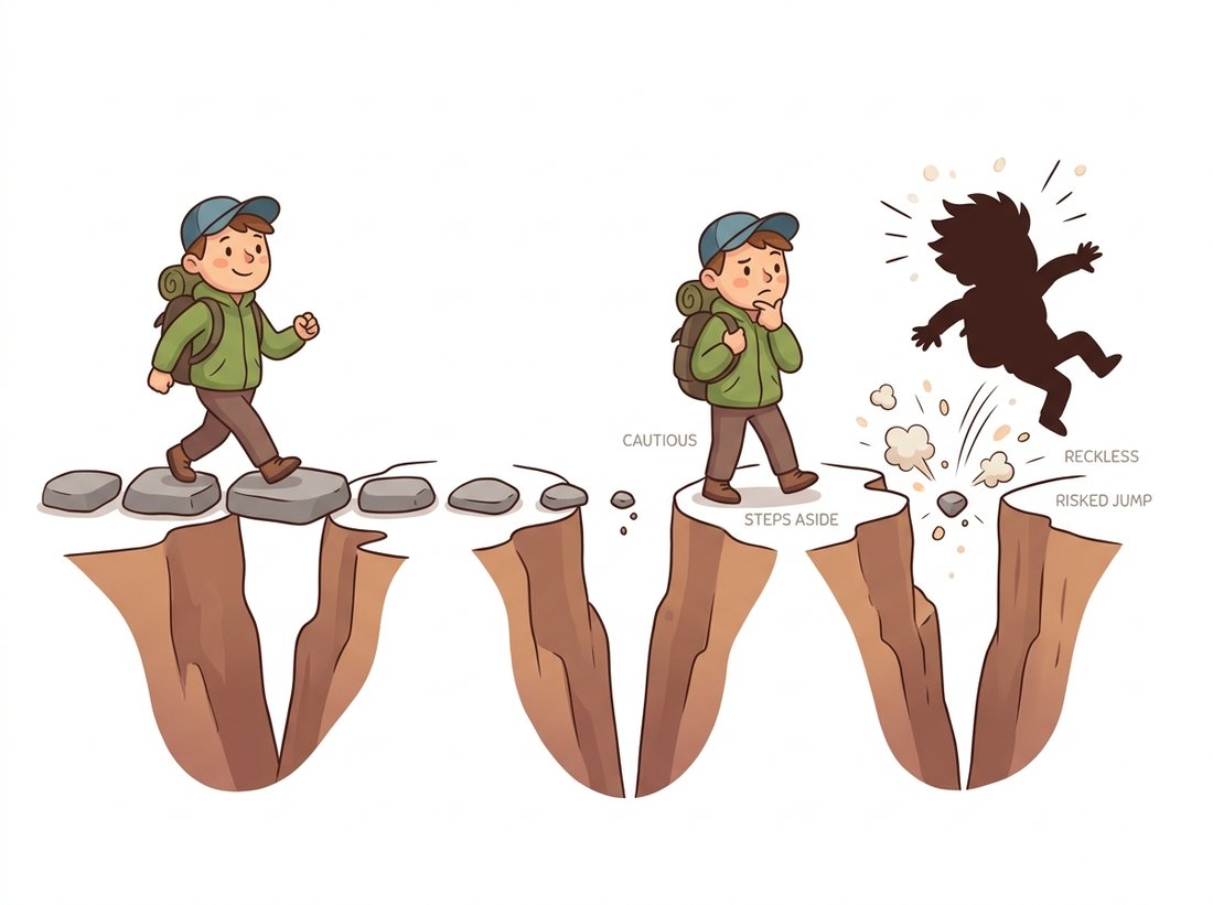
Section 7.2 fought the additive term in the degradation model $g = h \ast f + n$. This section fights the convolution. Blur is in some ways a kinder enemy than noise: it is deterministic, it destroys no pixels outright, and if you know the kernel $h$ exactly, the damage is in principle reversible. The phrase "in principle" is where three decades of engineering live, because the reversal is the most spectacularly ill-posed operation in this chapter, and noise, even a whisper of it, is what makes it so.

1. A Gallery of Point Spread Functions Beginner

The blur kernel $h$ has a physical name, the point spread function: it is literally the image that a single point of light produces after passing through your optics. Section 7.1 placed it in the degradation pipeline; here we meet the three shapes that cover most of practice. A defocused lens spreads a point into a filled disk (the aperture's shape, which is why out-of-focus highlights look like little polygons matching the iris blades). Camera shake or subject motion during the exposure drags the point along a path, in the simplest case a straight line whose length and angle encode the motion. And the combined small imperfections of atmosphere, diffraction, and lens design aggregate into something well approximated by the Gaussian kernel of Chapter 3. Code 7.3.1 builds the motion case, which we will use as the running example.

import numpy as np
from scipy.signal import fftconvolve
from skimage import data, img_as_float
from skimage.metrics import peak_signal_noise_ratio as psnr

def motion_psf(length=15, angle_deg=30, size=31):
    """Line PSF: a 1-pixel-wide segment of given length and angle,
    normalized to sum to 1 (blur must conserve brightness)."""
    psf = np.zeros((size, size))
    c = size // 2
    a = np.deg2rad(angle_deg)
    for t in np.linspace(-length / 2, length / 2, 4 * length):
        i = int(round(c + t * np.sin(a)))
        j = int(round(c + t * np.cos(a)))
        psf[i, j] = 1.0
    return psf / psf.sum()

rng = np.random.default_rng(seed=7)
clean = img_as_float(data.camera())
psf = motion_psf()
blurred = fftconvolve(clean, psf, mode='same')
noisy_blurred = np.clip(blurred + rng.normal(0, 0.005, clean.shape), 0, 1)
print(f"blurred PSNR vs clean: {psnr(clean, noisy_blurred):.1f} dB")

In real systems you obtain the PSF rather than assume it: astronomers read it off stars (genuine point sources), microscopists image sub-resolution fluorescent beads, and lens labs photograph backlit pinholes or slanted edges. When none of that is possible, the PSF must be estimated from the blurred image itself, the "blind" problem we defer to Section 5. For now, assume $h$ is known and exact.

2. The Inverse Filter Catastrophe Intermediate

The convolution theorem from Chapter 4 turns the degradation model into per-frequency multiplication: $G(u,v) = H(u,v)\,F(u,v) + N(u,v)$, where capital letters are Fourier transforms. Solving for the unknown image looks like one line of algebra:

The first term is exactly what we want, the true image, fully recovered. The second term is the catastrophe. A blur kernel is an averaging operation, so $H$ falls toward zero at high frequencies, and a line-shaped motion PSF is worse: its transform is a sinc-like pattern that crosses zero repeatedly throughout the frequency plane. At every such frequency we are dividing the noise, which is flat and indifferent, by a number arbitrarily close to zero. Figure 7.3.1 sketches the disaster and the remedy to come.

Code 7.3.2 commits the naive inversion so you can watch it fail. The noise we added is half a percent of the intensity range, far below visibility, yet the output is unrecognizable static. This is not an implementation bug; it is the textbook definition of an ill-posed inverse problem, and the single most important demonstration in this chapter.

def fft_of_psf(psf, shape):
    """Zero-pad the PSF to image size, center it, return its 2D FFT."""
    padded = np.zeros(shape)
    k = psf.shape[0]
    padded[:k, :k] = psf
    # roll so the PSF center sits at (0, 0), as the FFT convention expects
    padded = np.roll(padded, (-(k // 2), -(k // 2)), axis=(0, 1))
    return np.fft.fft2(padded)

H = fft_of_psf(psf, clean.shape)
G = np.fft.fft2(noisy_blurred)

F_naive = G / H                          # the one-line "solution"
restored_naive = np.real(np.fft.ifft2(F_naive))
print(f"inverse filter PSNR: {psnr(clean, np.clip(restored_naive, 0, 1)):.1f} dB")

inverse filter PSNR: 5.8 dB

3. The Wiener Filter: Divide Only Where It Pays Intermediate

The fix is to stop demanding exact inversion and ask instead for the linear filter that minimizes the expected squared error of the restoration, given the statistics of signal and noise. Norbert Wiener solved that problem in general; for our model the answer replaces $1/H$ with

where $H^*$ is the complex conjugate and $K$ is the noise-to-signal power ratio at each frequency. Read it as a negotiation. Where the blurred signal towers over the noise ($|H|^2 \gg K$), the filter behaves like the exact inverse $1/H$. Where blur has crushed the signal below the noise floor ($|H|^2 \ll K$), the denominator is dominated by $K$ and the gain glides to zero: those frequencies are abandoned rather than amplified, which is precisely the green curve of Figure 7.3.1. In practice nobody knows the true power spectra, so $K$ is collapsed to a single constant and tuned, which makes it this method's one honest knob. Code 7.3.3 implements the whole thing in six lines and sweeps the knob.

def wiener_deconv(g, H, K):
    """Wiener deconvolution with a constant noise-to-signal ratio K."""
    G = np.fft.fft2(g)
    W = np.conj(H) / (np.abs(H) ** 2 + K)
    return np.clip(np.real(np.fft.ifft2(W * G)), 0, 1)

for K in [1e-1, 1e-2, 1e-3, 1e-4]:
    out = wiener_deconv(noisy_blurred, H, K)
    print(f"K = {K:.0e}   PSNR = {psnr(clean, out):.1f} dB")

K = 1e-01   PSNR = 24.8 dB
K = 1e-02   PSNR = 26.7 dB
K = 1e-03   PSNR = 28.4 dB
K = 1e-04   PSNR = 26.0 dB

The visual signature of Wiener restoration is worth knowing: crisp recovered edges accompanied by faint ringing, ripples parallel to strong edges at the frequencies the filter gave up on. Ringing is not a bug but a receipt, the visible cost of the frequencies that were surrendered to noise. Heavier-handed priors (total variation deconvolution, which penalizes gradient magnitude, is the classic upgrade) trade ringing for staircase flatness; every deconvolution method leaves a fingerprint.

from skimage.restoration import wiener, unsupervised_wiener

restored_w = wiener(noisy_blurred, psf, balance=0.01)
restored_u, _ = unsupervised_wiener(noisy_blurred, psf)   # tunes itself

4. Richardson-Lucy: Deconvolution for Photon Counters Advanced

The Wiener filter assumes additive Gaussian noise, but Section 7.1 taught that photon-limited images, astronomy, fluorescence microscopy, low-dose X-ray, obey Poisson statistics, where the noise scales with the signal. Richardson (1972) and Lucy (1974), working independently, derived the maximum-likelihood estimate for exactly that case. The result is not a closed form but a beautifully simple fixed-point iteration:

where $h^{\dagger}$ is the PSF flipped in both axes. The loop reads like a conversation. Blur your current guess ($h \ast f^{(k)}$) and compare it to what the camera actually saw, as a ratio: 1 where the guess explains the data, above 1 where the guess is too dim, below 1 where too bright. Smear that ratio backward through the optics ($h^{\dagger} \ast$) so each source pixel hears about the mismatches it could have caused, then scale the guess multiplicatively. The multiplicative update has two elegant consequences: a nonnegative guess stays nonnegative forever (no negative light, a constraint Wiener cheerfully violates), and total flux is conserved, which is why astronomers trust it for photometry. Code 7.3.5 is the entire algorithm.

def richardson_lucy_scratch(g, psf, n_iter=30):
    """Richardson-Lucy deconvolution, the whole algorithm."""
    f = np.full(g.shape, 0.5)                 # flat, positive initial guess
    psf_flipped = psf[::-1, ::-1]
    for _ in range(n_iter):
        estimate = fftconvolve(f, psf, mode='same')
        ratio = g / (estimate + 1e-12)        # observed vs predicted
        f = f * fftconvolve(ratio, psf_flipped, mode='same')
    return np.clip(f, 0, 1)

for n in [5, 15, 30, 80]:
    out = richardson_lucy_scratch(noisy_blurred, psf, n_iter=n)
    print(f"{n:3d} iterations   PSNR = {psnr(clean, out):.1f} dB")

  5 iterations   PSNR = 25.9 dB
 15 iterations   PSNR = 27.8 dB
 30 iterations   PSNR = 28.3 dB
 80 iterations   PSNR = 26.9 dB

Semi-convergence is the Richardson-Lucy version of the Wiener knob: the iteration count is the regularization. Stop early and you accept residual blur; run long and you amplify noise, just more gracefully than the inverse filter did. Production variants add explicit damping or a total-variation penalty inside the loop so the iteration can run to convergence safely. The library one-liner, skimage.restoration.richardson_lucy(noisy_blurred, psf, num_iter=30), implements the same loop with the same semantics, and is the version to use outside teaching.

5. Blind Deconvolution and the Real World Advanced

When the PSF cannot be measured, it must be estimated from the blurred image itself, jointly with the image: the blind deconvolution problem, which is doubly ill-posed (a sharp image with wide blur and a blurry image with narrow blur explain the data equally well; so does the original photo of an intrinsically blurry scene). Classical practice tames it with structure. For straight-line motion blur, the PSF has only two parameters, and the blur's periodic zero crossings (Figure 7.3.1) leave measurable notches in the image's power spectrum from which length and angle can be read, a trick built on the cepstrum. For defocus, the disk radius is a one-parameter search scored by how natural the deconvolution result looks. General blind methods alternate between updating the image given the PSF and the PSF given the image, each step a constrained Richardson-Lucy-like update; they work, fragilely, and they are the part of this section that deep learning improved first and most.