"Every photon is a coin flip and every electron has an opinion. I just write down the average and hope you call it a photograph."
A Statistically Honest Image Sensor
You cannot undo damage you cannot describe: every restoration algorithm begins as a forward model of how the clean image became the dirty one. This section builds that forward model piece by piece, from the quantum randomness of photon arrival to the blur of optics and the artifacts of compression, because the quality of every denoiser, deblurrer, and super-resolver in this chapter is bounded by the fidelity of the degradation model it assumes.
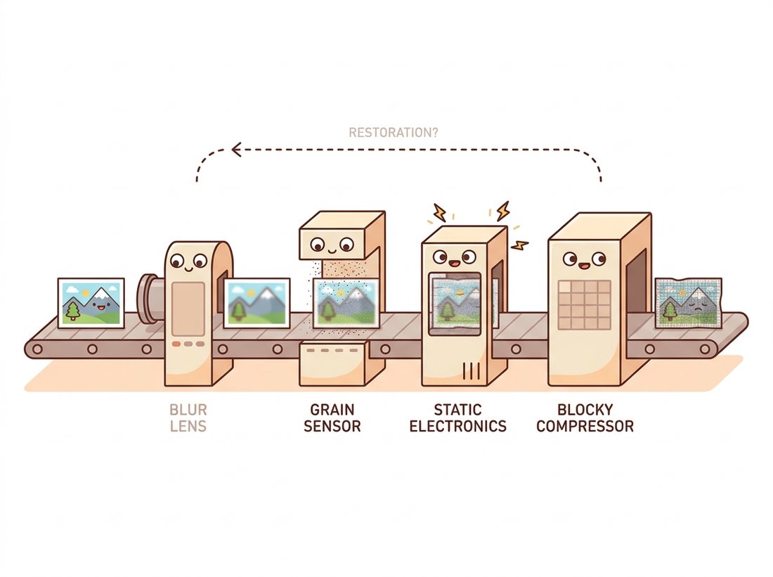
In Chapter 6 we enjoyed the luxury of clean binary images, where every pixel was confidently foreground or background. That luxury was manufactured: real images arrive damaged, and pretending otherwise is how pipelines fail in production. This section opens the restoration chapter by studying the damage itself. Before asking "how do I remove noise?" we ask the better questions: what process generated the noise, what statistical signature does it carry, and how can we reproduce it faithfully enough to test our cures? Think of the whole chapter as a patient repair shop (see the illustration below), where the cure always begins by naming the damage.

1. The Degradation Model Beginner
Nearly every problem in this chapter fits a single equation. Let $f(x, y)$ be the ideal image we wish we had captured, $h(x, y)$ a blur kernel called the point spread function (PSF), $\ast$ the convolution we built in Chapter 3, and $n(x, y)$ a random noise field. The observed image is
$$ g(x, y) = (h \ast f)(x, y) + n(x, y). $$Restoration is the attempt to recover $f$ from $g$, given whatever we know about $h$ and the statistics of $n$. Stated this way, the problem looks like algebra: subtract the noise, divide out the blur. The reason this chapter exists is that both steps are treacherous. The noise is random, so it cannot be subtracted, only suppressed at the cost of some signal. The blur, viewed in the frequency domain of Chapter 4, multiplies some frequencies by numbers close to zero, and dividing by almost-zero amplifies whatever noise lives there. Restoration problems are ill-posed: many candidate images $f$ explain the observation $g$ essentially equally well, and picking among them requires assumptions about what images look like, assumptions this book will call priors.
Figure 7.1.1 traces the full journey from scene to file, with each stage contributing its own term to the model. The pipeline mirrors the camera hardware tour of Chapter 1, but now with an accountant's eye: every box is a place where information is lost, and every loss has a statistical fingerprint. The friendly assembly line below makes the same point before the formal schematic does.
2. A Field Guide to Noise Intermediate
"Noise" is not one thing. The label covers several physically distinct random processes, and each demands different treatment. The four entries below cover the vast majority of what you will meet in practice; Table 7.1.1 summarizes their signatures.
Photon shot noise. Light is quantized. A pixel that "should" collect 100 photons during the exposure actually collects a Poisson-distributed count: sometimes 91, sometimes 107. The Poisson distribution's defining property is that its variance equals its mean, so a pixel collecting $\lambda$ photons fluctuates with standard deviation $\sqrt{\lambda}$. This has a consequence worth memorizing: bright pixels are noisier in absolute terms but cleaner in relative terms, since the signal-to-noise ratio is $\lambda / \sqrt{\lambda} = \sqrt{\lambda}$. Shot noise is not a defect of the sensor; it is a property of light itself, and no hardware will ever remove it.
Read noise. Converting accumulated charge to a digital number involves amplifiers and an analog-to-digital converter, all of which add small, signal-independent fluctuations. Read noise is well modeled as zero-mean Gaussian noise with a fixed standard deviation, and it dominates in the darkest regions of an image, where the photon count is too small for shot noise to matter. This is why the shadows of a night photo look grainy while the bright window in the same frame looks clean.
Impulse (salt-and-pepper) noise. Dead or hot pixels, transmission bit errors, and certain sensor defects replace individual pixels with extreme values: full black or full white. The defining feature is that affected pixels carry no information at all about the true value; the median filter from Chapter 3 is the classical cure precisely because it discards extreme values rather than averaging them in.
Speckle. Coherent imaging systems, including ultrasound, synthetic aperture radar, and laser imaging, produce multiplicative noise: the noise amplitude scales with the signal, $g = f + f \cdot n$. Multiplicative noise turns into additive noise under a logarithm, which is the standard preprocessing trick in those fields.
| Noise | Model | Signal-dependent? | Typical source | Classical cure |
|---|---|---|---|---|
| Shot (photon) | Poisson, $\sigma^2 = \lambda$ | yes | quantum nature of light | averaging, variance stabilization |
| Read | Gaussian, fixed $\sigma$ | no | amplifier and ADC electronics | any linear or patch denoiser |
| Salt-and-pepper | impulse, $p$ corrupted | no | dead pixels, bit errors | median filter |
| Speckle | multiplicative, $g = f(1+n)$ | yes | coherent imaging (ultrasound, SAR) | log transform, then denoise |
| Quantization | uniform, $\pm \tfrac{1}{2}$ LSB | no | finite bit depth | dithering, higher bit depth |
Two more degradations deserve membership in the field guide even though they are not "noise" in the random sense. Quantization rounds continuous values to the nearest of $2^b$ levels, contributing a small uniform error and, at low bit depths, visible banding (recall the bit-depth experiments of Chapter 1). And JPEG compression introduces structured, deterministic artifacts: 8x8 blocking and ringing around edges, which behave nothing like random noise and defeat denoisers designed for it. A restoration pipeline that ignores compression artifacts will faithfully "denoise" the blocking pattern into the output.
Mismatching the noise model costs more than choosing a mediocre denoiser. A Gaussian-noise denoiser applied to salt-and-pepper noise smears the impulses into blobs instead of removing them; applied to Poisson noise, it over-smooths shadows and under-smooths highlights because it assumes one global $\sigma$ where the truth varies per pixel. Before reaching for any algorithm in Section 7.2, identify the dominant noise source. The cure follows from the diagnosis, rarely the other way around.
The diagnose-then-cure discipline compresses into four pairings worth memorizing, one per common noise. Grain that grows with brightness means shot (Poisson) noise: stabilize, then denoise. Grain only in the shadows means read (Gaussian) noise: any linear or patch denoiser. Isolated black or white specks means impulse noise: take a median, never an average. Grain that scales with the signal in a coherent scan means speckle: take a logarithm first. The shape of the noise names its own cure; the algorithm is the easy part once the diagnosis is right.
3. Synthesizing Noise in Code Intermediate
Restoration research has a peculiar advantage over most of vision: you can manufacture perfect ground truth. Take a clean image, damage it with a known model, restore it, and compare against the original with the PSNR and SSIM metrics from Chapter 1. Everything in this chapter is evaluated that way, so our first piece of code, Code 7.1.1, is the damage generator itself.
# Four noise generators, one per row of Table 7.1.1.
# All take and return float images in [0, 1]; a fixed seed keeps runs reproducible.
import numpy as np

rng = np.random.default_rng(seed=7)

def add_gaussian(img, sigma=0.05):
    """Additive read-noise model. img is float in [0, 1]."""
    return np.clip(img + rng.normal(0, sigma, img.shape), 0, 1)

def add_poisson(img, peak=100.0):
    """Shot noise: scale to 'peak' photons, draw Poisson counts, rescale."""
    photons = rng.poisson(img * peak)          # variance == mean, per pixel
    return np.clip(photons / peak, 0, 1)

def add_salt_pepper(img, amount=0.02):
    """Impulse noise: a fraction 'amount' of pixels forced to 0 or 1."""
    out = img.copy()
    coords = rng.random(img.shape)
    out[coords < amount / 2] = 0.0             # pepper
    out[coords > 1 - amount / 2] = 1.0         # salt
    return out

def add_speckle(img, sigma=0.15):
    """Multiplicative noise: g = f * (1 + n)."""
    return np.clip(img * (1 + rng.normal(0, sigma, img.shape)), 0, 1)
The Poisson generator deserves a second look because it is the one that trips people up. There is no "Poisson noise array" to add: the image itself parameterizes the distribution, pixel by pixel. The peak argument sets how many photons the brightest pixel collects, and it is the single dial controlling noise severity. A peak of 10,000 simulates a sunny day (nearly invisible noise); a peak of 30 simulates a dim interior, and the shadows fall apart exactly the way they do in a real night shot.
skimage.util.random_noiseThe four generators above, plus localvar and Poisson variants and all the clipping bookkeeping, ship as one function in scikit-image:
from skimage.util import random_noise

noisy_g  = random_noise(img, mode='gaussian', var=0.05**2)
noisy_p  = random_noise(img, mode='poisson')
noisy_sp = random_noise(img, mode='s&p', amount=0.02)
noisy_sk = random_noise(img, mode='speckle', var=0.15**2)
random_noise. One mode string selects the model and the library handles float conversion, Poisson rescaling, seeding, and clipping internally.Roughly 25 lines of generator code become 4 calls. Internally the library handles float conversion, the rescaling conventions for Poisson mode, seed management, and clipping, the exact bookkeeping that produces subtle bugs when hand-rolled. Keep the from-scratch versions for understanding; use this one in pipelines.
4. Signal-Dependent Noise & Variance Stabilization Advanced
Real sensor noise is a mixture: Poisson shot noise plus Gaussian read noise, often summarized as the Poisson-Gaussian model. Its variance is an affine function of the true signal,
$$ \operatorname{Var}[g(x,y)] = a \, f(x, y) + b, $$where $a$ reflects the sensor gain (the Poisson part) and $b$ the read-noise floor (the Gaussian part). This signal dependence is awkward: nearly every classical denoiser in Section 7.2 assumes one global noise level. The classical workaround is elegant. A variance-stabilizing transform remaps intensities so that the noise becomes approximately uniform across the range. For pure Poisson data the standard choice is the Anscombe transform,
$$ A(x) = 2\sqrt{x + \tfrac{3}{8}}, $$which converts Poisson noise of any mean into approximately unit-variance Gaussian noise. The recipe, demonstrated in Code 7.1.3, is a sandwich: transform, denoise with any Gaussian-noise method, transform back. The inverse must be applied carefully (the naive algebraic inverse is biased for small counts; libraries provide the corrected "exact unbiased" inverse), but the sandwich pattern itself is universal and reappears throughout imaging science.
def anscombe(x):
    return 2.0 * np.sqrt(x + 3.0 / 8.0)

def inverse_anscombe(y):
    # Simple algebraic inverse; biased at very low counts.
    return (y / 2.0) ** 2 - 3.0 / 8.0

photons = rng.poisson(img * 30.0)              # severe low-light shot noise

stabilized = anscombe(photons)
print(f"dark-region std:   {stabilized[img < 0.2].std():.3f}")
print(f"bright-region std: {stabilized[img > 0.8].std():.3f}")
# Both stds are now close to 1.0; before stabilization the bright
# regions had ~5x the standard deviation of the dark ones.
Who: An imaging engineer at a dental X-ray equipment manufacturer.
Situation: Marketing wanted diagnostic-quality images at 30 percent lower radiation dose, which means 30 percent fewer photons and visibly stronger noise.
Problem: The team's first attempt applied a well-tuned Gaussian denoiser uniformly. Radiologists rejected the result: fine trabecular bone texture was smeared away in bright regions while dark regions still crawled with residual noise. The single global sigma was simultaneously too aggressive and too timid.
Decision: An analysis of flat calibration exposures showed variance growing linearly with intensity, the signature of photon-limited imaging. The engineer inserted an Anscombe transform before the existing denoiser and the corrected inverse after it, changing fewer than twenty lines of code.
Result: The same denoiser, now operating on stabilized data, passed the radiologist review at the reduced dose. No new denoising algorithm was needed.
Lesson: When a denoiser fails differently in dark and bright regions, suspect the noise model before the denoiser. Signal-dependent noise wants stabilization, not stronger filtering.
5. Estimating Noise From a Single Image Intermediate
Synthetic experiments hand you $\sigma$; real images do not. Most denoisers need a noise-level estimate, and getting one from the noisy image itself is a small art. The intuition: in a perfectly flat region, all variation is noise, so the local standard deviation there estimates $\sigma$ directly. The classical automated estimator (due to Donoho and Johnstone's wavelet work) is the median absolute deviation of the finest wavelet detail coefficients (the wavelet transform and its detail coefficients were built in Section 4.6), which sees mostly noise and is robust to the minority of coefficients carrying real edges. Code 7.1.4 compares the flat-patch idea against scikit-image's wavelet estimator.
from skimage.restoration import estimate_sigma
from skimage import data, img_as_float

clean = img_as_float(data.camera())            # 512x512 grayscale test image
noisy = add_gaussian(clean, sigma=0.08)

# Manual estimate: standard deviation inside a visually flat patch (sky).
flat_patch = noisy[10:60, 200:300]
print(f"flat-patch estimate: {flat_patch.std():.4f}")

# Automated wavelet-based estimate over the whole image.
print(f"estimate_sigma:      {estimate_sigma(noisy):.4f}")
flat-patch estimate: 0.0807
estimate_sigma:      0.0792
6. Degradation Pipelines: Damage as a Product Intermediate
Single degradations are for textbooks. A photo shared on a messaging app has been blurred by optics, shot-noised by the sensor, denoised badly by the phone's image signal processor (ISP), downscaled, and JPEG-compressed twice. Restoration methods tuned for one pristine degradation routinely collapse on such compound damage. The modern response, which began in classical restoration and became the foundation of deep "blind" restoration, is to model degradation as a pipeline: a composition of randomized stages. Code 7.1.5 builds a representative one.
import cv2

def degrade(img_u8, rng):
    """Compound degradation: blur -> downscale -> noise -> JPEG.
    img_u8: uint8 BGR image. Returns a damaged uint8 image, same size."""
    h, w = img_u8.shape[:2]

    # 1. Optical blur with a random kernel width
    k = rng.choice([3, 5, 7])
    out = cv2.GaussianBlur(img_u8, (k, k), 0)

    # 2. Downscale and re-upscale (resolution loss), random factor
    s = rng.uniform(0.4, 0.8)
    small = cv2.resize(out, None, fx=s, fy=s, interpolation=cv2.INTER_AREA)
    out = cv2.resize(small, (w, h), interpolation=cv2.INTER_LINEAR)

    # 3. Sensor noise (Gaussian, random strength)
    sigma = rng.uniform(2, 12)                  # in 8-bit units
    out = np.clip(out + rng.normal(0, sigma, out.shape), 0, 255).astype(np.uint8)

    # 4. JPEG round trip at a random quality
    q = int(rng.uniform(35, 90))
    ok, buf = cv2.imencode('.jpg', out, [cv2.IMWRITE_JPEG_QUALITY, q])
    return cv2.imdecode(buf, cv2.IMREAD_COLOR)
The randomization is the point. If you evaluate (or train) against one fixed degradation, you learn to invert that one recipe and nothing else. Sampling kernel widths, scales, noise levels, and JPEG qualities forces robustness across the whole neighborhood of plausible damage. This is precisely the idea that powers Real-ESRGAN's "high-order" degradation modeling: apply a pipeline like Code 7.1.5 twice in a row, and synthetic training data starts to resemble genuine internet-quality damage. We will reuse this generator when we evaluate denoisers in Section 7.2 and super-resolvers in Section 7.5; the same philosophy of randomized corruption returns as data augmentation in Chapter 21.
The most consequential noise generator of the 2020s is six lines long. Diffusion models, the engines behind modern image generators covered in Chapter 33, train by deliberately adding Gaussian noise to clean images at a thousand graduated severities and learning to undo each step. The "noise schedule" they tune so carefully is, in the vocabulary of this section, just a parameterized family of add_gaussian calls. Damage synthesis grew up to become a generative industry.
7. Scoring the Cure Beginner
One final piece of apparatus before the cures begin. Throughout this chapter we score restorations with the fidelity metrics introduced in Chapter 1: PSNR, which is a logarithmic repackaging of mean squared error, and SSIM, which compares local structure. Both require ground truth, which is why the synthetic degradation pipeline above matters so much. Keep two caveats in mind. First, PSNR rewards blur: an over-smoothed image often outscores a sharper one with mild residual noise, because squared error punishes outliers more than mush. Second, neither metric measures plausibility, which becomes the dominant criterion for inpainting in Section 7.4 and for generative restoration later in the book. Use the numbers, but look at the pictures. With the damage modeled, synthesized, and scorable, the rest of the chapter turns to the cures, beginning with the oldest and most intuitive: averaging noise away in Section 7.2.
The frontier of restoration research in 2024 through 2026 is less about new denoisers and more about degradation realism. Real-ESRGAN (Wang et al., 2021) showed that a restorer trained purely on synthetic compound degradations generalizes to real photos, making the degradation pipeline itself the core intellectual property. DiffBIR (Lin et al., ECCV 2024) splits blind restoration into two stages, degradation removal followed by a generative diffusion prior, while SUPIR (Yu et al., CVPR 2024) scales the same recipe to a multi-billion-parameter prior that can reconstruct convincingly from near-total destruction. The open question these systems sharpen: when the prior is that strong, the output is no longer evidence of what the pixels were, only of what they plausibly could have been, a distinction that matters enormously for forensic and medical use.
For each scenario, name the dominant degradation from Table 7.1.1 and justify your answer in one sentence: (a) a security camera image at night with grainy shadows but clean bright areas around streetlights; (b) an old scanned photograph with isolated pure-white specks; (c) an ultrasound scan whose noise is strongest in the brightest tissue; (d) a meme that has been re-shared many times and shows faint 8x8 grid seams; (e) a smooth sky gradient that shows visible stripes of constant color.
Using Code 7.1.1 as a starting point, write a function that takes a clean image and produces a labeled grid of its Gaussian, Poisson, salt-and-pepper, and speckle corruptions at three severities each. For every cell, compute PSNR against the clean original. Then verify your Poisson implementation: for peak values of 30, 100, and 1000, plot per-pixel sample variance against mean intensity (bin pixels by intensity) and confirm the relationship is linear through the origin.
Corrupt a clean image with strong Poisson noise (peak=25). Denoise it two ways: (a) directly with a Gaussian blur of the best sigma you can find by sweeping; (b) with the Anscombe sandwich of Code 7.1.3 around the same sweep. Report the best PSNR of each route and, more importantly, compare crops of a dark region and a bright region. Explain the visual difference using the variance formula $\operatorname{Var} = a f + b$.