Classical Super-Resolution

"One frame is a rumor. Eight frames with sub-pixel shifts are a sworn deposition, and I am the court stenographer."

A Meticulous Multi-Frame Super-Resolver

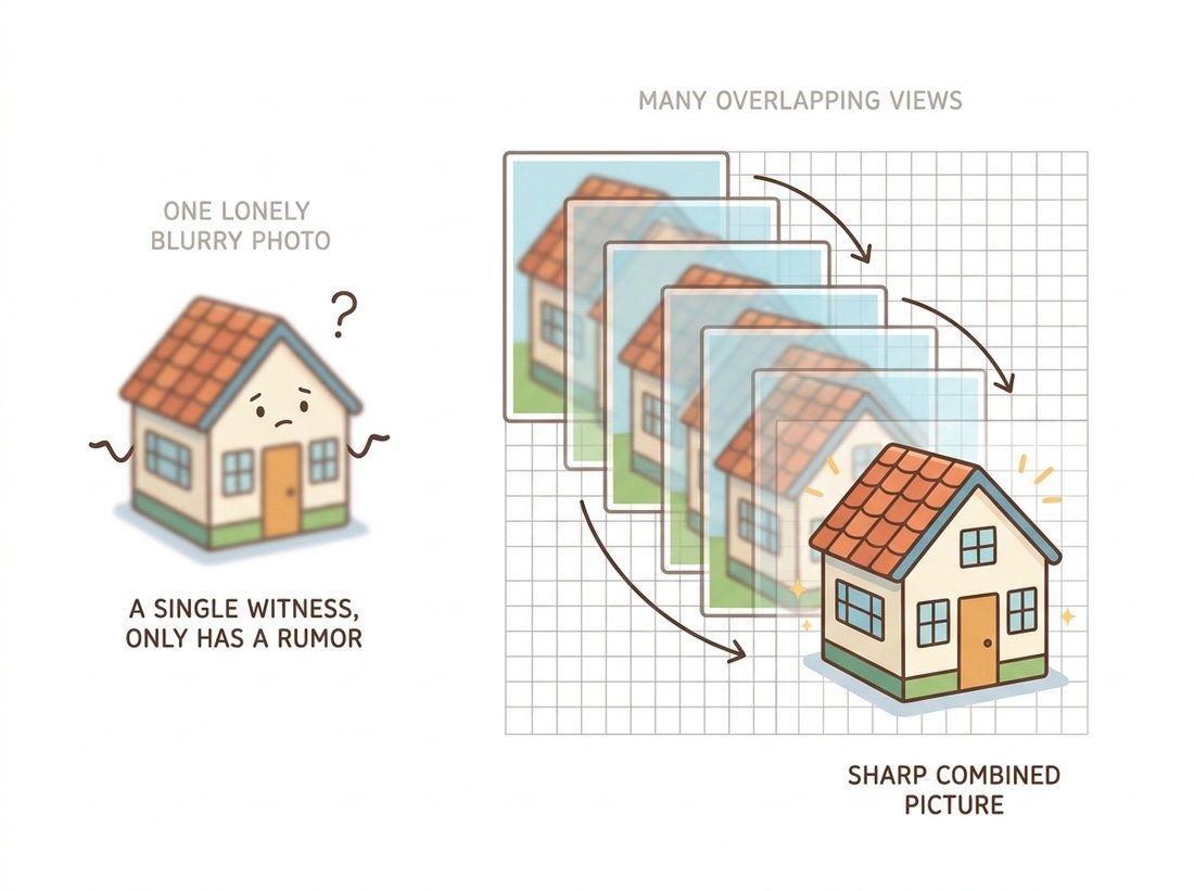
The previous sections repaired pixels that were noisy (Section 7.2), smeared (Section 7.3), or missing (Section 7.4). This section asks for pixels that were never captured at all: given a low-resolution image, produce a higher-resolution one. Phrased that way it sounds impossible, and for a single image, in the strict information-theoretic sense, it is. The classical escape is to stop asking one image to do it. Before deep networks learned to hallucinate plausible detail, super-resolution meant honest accounting: finding measurements that genuinely exist, scattered across multiple frames, and assembling them.

1. Adding Pixels Is Not Adding Information Beginner

Chapter 5 built the interpolation toolbox: bilinear, bicubic, Lanczos. All of them can resize an image to any dimensions you like, and none of them perform super-resolution. The sampling theorem from Chapter 4 says why: a grid of $N \times N$ samples can represent spatial frequencies up to its Nyquist limit and nothing above. Interpolating to $2N \times 2N$ creates new pixel values, but every one of them is a weighted average of the original samples; the spectrum gains no content beyond the original Nyquist limit. The result is larger, smoother, and exactly as informative. Upscaled text remains unreadable at any size, just more politely blurred.

So where could genuinely new information come from? Three honest sources exist: more measurements of the same scene (multiple frames, the core of this section), prior knowledge about the scene's structure (the example-based methods of Section 5), and knowledge of the camera's own blur (folding in the deconvolution of Section 7.3). Everything classical is some mix of the three.

2. The Observation Model, and Aliasing the Ally Intermediate

As always in this chapter, the cure starts with a forward model. Let $x$ be the high-resolution (HR) image we want, and let each captured low-resolution (LR) frame $y_k$ be produced by warping, blurring, and downsampling it:

where $W_k$ is a geometric warp (for handheld video, nearly a pure translation between consecutive frames), $B$ is the camera blur from Section 7.3, $D$ is decimation to the coarse grid, and $n_k$ is noise from Section 7.1. Each frame is a different set of linear equations about the same unknown $x$; collect enough independent equations and the system becomes solvable. The independence comes from the warps: if frame $k$ is shifted by half an LR pixel relative to frame $j$, its sensor wells integrate different parts of the scene, and its equations are new.

Here is the counterintuitive heart of the subject: this only works if the LR frames are aliased. Chapter 4 presented aliasing as a sin: frequencies above Nyquist fold down and masquerade as low frequencies. But masquerading information is still information. In an aliased frame, the high frequencies of the scene are present, folded and entangled with the low ones; different sub-pixel shifts entangle them with different phases, and a set of differently-shifted frames gives you the linear system that disentangles them. A camera with a perfect anti-aliasing filter destroys those high frequencies before sampling, and then no quantity of frames can recover them: the equations all say the same thing. Figure 7.5.1 shows the mechanics on the sampling grid.

3. Shift-and-Add: Super-Resolution by Bookkeeping Intermediate

The simplest fusion algorithm follows Figure 7.5.1 literally. Estimate each frame's shift relative to a reference, scale the shifts up to the fine grid, then deposit every LR pixel onto its registered fine-grid position and average whatever lands in each bin. Registration must be sub-pixel accurate, and Chapter 4 already supplied the tool: phase correlation, which reads translation off the Fourier phase difference and, with local upsampling of the correlation peak, resolves shifts to a few hundredths of a pixel. Code 7.5.1 runs the full pipeline on synthetic frames so the gain over bicubic is measurable.

import numpy as np
import cv2
from scipy.ndimage import shift as nd_shift
from skimage import data, img_as_float
from skimage.registration import phase_cross_correlation
from skimage.metrics import peak_signal_noise_ratio as psnr

rng = np.random.default_rng(seed=7)
hr = img_as_float(data.camera())                  # ground-truth HR, 512x512
SCALE = 2

def capture_lr(hr_img, dy, dx):
    """One observation: sub-pixel shift, mild blur, decimate, noise."""
    shifted = nd_shift(hr_img, (dy, dx), order=3, mode='reflect')
    blurred = cv2.GaussianBlur(shifted, (3, 3), 0.6)
    lr = blurred[::SCALE, ::SCALE]                # decimation keeps aliasing!
    return np.clip(lr + rng.normal(0, 0.01, lr.shape), 0, 1)

true_shifts = [(0.0, 0.0)] + [tuple(rng.uniform(0, SCALE, 2)) for _ in range(7)]
frames = [capture_lr(hr, dy, dx) for dy, dx in true_shifts]

# --- Register every frame to frame 0, to sub-pixel precision ---
est = [phase_cross_correlation(frames[0], f, upsample_factor=50)[0]
       for f in frames]                           # shift in LR pixels

# --- Deposit samples onto the fine grid, average per bin ---
acc  = np.zeros(hr.shape)
hits = np.zeros(hr.shape)
for f, (sy, sx) in zip(frames, est):
    ys = (np.arange(f.shape[0]) * SCALE - sy * SCALE).round().astype(int)
    xs = (np.arange(f.shape[1]) * SCALE - sx * SCALE).round().astype(int)
    yy, xx = np.meshgrid(ys % hr.shape[0], xs % hr.shape[1], indexing='ij')
    np.add.at(acc,  (yy, xx), f)
    np.add.at(hits, (yy, xx), 1)

fused = np.where(hits > 0, acc / np.maximum(hits, 1), 0)
empty = hits == 0                                 # fine-grid bins nobody hit
fused[empty] = cv2.resize(frames[0], hr.shape[::-1],
                          interpolation=cv2.INTER_CUBIC)[empty]

bicubic = cv2.resize(frames[0], hr.shape[::-1], interpolation=cv2.INTER_CUBIC)
print(f"bicubic x2 (1 frame):    PSNR = {psnr(hr, bicubic):.1f} dB")
print(f"shift-and-add (8 frames): PSNR = {psnr(hr, fused):.1f} dB")

bicubic x2 (1 frame):    PSNR = 27.5 dB
shift-and-add (8 frames): PSNR = 31.2 dB

4. Iterative Back-Projection: Simulate, Compare, Correct Advanced

Shift-and-add ignores two terms of the observation model: the blur $B$, and the fact that an LR pixel is an average over a fine-grid neighborhood rather than a point sample. Irani and Peleg's iterative back-projection (1991) honors the full model with a loop you have already met twice in this chapter: guess the HR image, push the guess forward through the model to simulate every LR frame, compare against the real frames, and push the errors backward to correct the guess. Formally,

where $U_k$ upsamples each residual and routes it back through the inverse warp. Code 7.5.2 implements it compactly, seeding the loop with the shift-and-add result.

def simulate_lr(x, sy, sx):
    """The forward model for frame k, matching capture_lr (minus noise)."""
    warped = nd_shift(x, (sy * SCALE, sx * SCALE), order=3, mode='reflect')
    return cv2.GaussianBlur(warped, (3, 3), 0.6)[::SCALE, ::SCALE]

x_hat = fused.copy()
for _ in range(15):
    correction = np.zeros_like(x_hat)
    for f, (sy, sx) in zip(frames, est):
        residual = f - simulate_lr(x_hat, sy, sx)         # what we got wrong
        up = cv2.resize(residual, x_hat.shape[::-1],
                        interpolation=cv2.INTER_CUBIC)
        correction += nd_shift(up, (-sy * SCALE, -sx * SCALE),
                               order=3, mode='reflect')
    x_hat = np.clip(x_hat + correction / len(frames), 0, 1)

print(f"back-projection (15 iters): PSNR = {psnr(hr, x_hat):.1f} dB")

back-projection (15 iters): PSNR = 32.6 dB

5. Single-Image Routes, and the Bridge to Learning Intermediate

When only one image exists, the missing information must come from priors, and the classical era built a clear progression of them. Edge-directed methods sharpened interpolation by snapping it to detected contours: honest, mild gains. Example-based super-resolution (Freeman et al., 2002) was the conceptual leap: build a dictionary of corresponding (LR patch, HR patch) pairs from training images, then assemble the output by looking up each input patch's HR counterpart. Sparse-coding variants (Yang et al., 2010) made the dictionary compact and the lookup a convex optimization, and Glasner et al. (2009) showed the dictionary could come from the input image itself, exploiting the cross-scale self-similarity cousin of Section 7.2's patch prior. Read those pipelines closely, patch encoding, a learned mapping, patch aggregation, and you can see SRCNN (2015) coming: it replaced each hand-built stage with a convolutional layer trained end to end, outperformed every dictionary method, and ended the classical era in three layers. The arc from hand-crafted pipeline to learned network repeats across all of vision, and Chapter 28 picks up super-resolution's deep, efficiency-obsessed present.

from cv2 import dnn_superres                  # pip install opencv-contrib-python

sr = dnn_superres.DnnSuperResImpl_create()
sr.readModel('FSRCNN_x2.pb')                  # weights from the official repo
sr.setModel('fsrcnn', 2)
upscaled = sr.upsample(lr_bgr_uint8)          # uint8 BGR in, upscaled out

6. Honest Limits, and Why Honesty Matters Beginner

How far can multi-frame methods go? In principle, $N^2$ ideally-placed frames support an $N\times$ factor; in practice the budget is spent by three taxes. Registration error: fusing at 4x demands registration good to a quarter of an LR pixel, and errors blur exactly the detail being recovered. Noise: each fine-grid bin receives only a few samples, so the averaging that denoised at 2x thins out. And the optical blur $B$: once the lens itself cannot pass a frequency, no sampling cleverness retrieves it, the same hard wall as the spectral zeros of Section 7.3. Practical systems top out around 2x to 4x, and the literature's standard advice stands: past there, you are deblurring and denoising, not resolving.