The Hough Transform: Lines & Circles

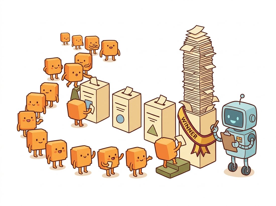
"I don't argue about where the line is. I hold an election and let every edge pixel vote. Turnout is excellent; the gaps never show up, and that's exactly the point."

A Hough Accumulator With Election-Night Energy

The previous section ended with the best edge map classical vision can produce: thin, well-localized, largely connected. But an edge map is still just pixels; nothing in it says "these 1,200 pixels form one straight line." This section builds the machine that says exactly that, first for lines, then for circles, and along the way introduces a way of thinking (transform the problem into parameter space, accumulate evidence, read off the peaks) that the curve fitting of Section 9.4 will complement and the lane detector of Section 9.5 will put to work.

1. The Grouping Problem Intermediate

Consider the naive approach first, because its failure explains the design. To find lines, you might trace contours: start at an edge pixel, follow its neighbors, and check whether the path stays straight. Tracing dies on contact with reality. Real edge maps have gaps (a shadow interrupts the curb), junctions (the curb crosses a lamp post), and clutter (leaves everywhere); a tracer must decide at every gap and junction what to do, and each decision compounds. Worse, tracing is sequential: one bad hop poisons everything after it.

The Hough transform inverts the logic. Instead of asking "which pixels chain together?", it asks each pixel independently: "which lines could you belong to?" Every edge pixel answers with a set of candidate lines, all candidates receive one vote each, and the lines that many pixels agree on win. No pixel ever needs to know about any other pixel; agreement emerges in the tally. Gaps cost nothing but a few missing votes, and clutter votes incoherently, scattering its ballots across parameter space without electing anyone.

2. Lines as Points: The $(\rho, \theta)$ Parameter Space Intermediate

To vote for a line you need an address for every line. The schoolbook form $y = mx + b$ fails the job: vertical lines need $m = \infty$, and near-vertical lines need enormous $m$, so no finite, evenly spaced ballot box can hold them. Duda and Hart's 1972 fix, now universal, addresses each line by its normal form:

$$ \rho = x \cos\theta + y \sin\theta, $$

where $\theta \in [0, \pi)$ is the direction of the line's normal and $\rho$ is the line's signed perpendicular distance from the origin. Every line in the image has exactly one $(\rho, \theta)$ address, both coordinates bounded: $\theta$ by construction, $\rho$ by the image diagonal $D$, so $\rho \in [-D, D]$. Vertical lines are nothing special ($\theta = 0$); the pathology is gone.

Now the elegant part. Fix an edge pixel $(x_0, y_0)$ and ask which lines pass through it: all $(\rho, \theta)$ satisfying $\rho = x_0 \cos\theta + y_0 \sin\theta$, which is a sinusoid in the $(\theta, \rho)$ plane. One pixel, one sinusoid. And if several pixels are collinear, their sinusoids all pass through the single $(\rho, \theta)$ address of the shared line: collinearity in the image becomes intersection in parameter space. Figure 9.3.1 draws the duality; it is the picture to hold in mind whenever Hough voting comes up.

3. Building the Accumulator From Scratch Advanced

Implementation is bookkeeping. Discretize parameter space into bins (say 1 degree by 1 pixel; for a 640×480 image that is 180 columns and about 1,600 rows, under 300k cells), give every edge pixel a vote in each $\theta$ column at the $\rho$ its sinusoid passes through, and find cells whose counts are both large and locally maximal. The code below vectorizes the votes with NumPy and verifies the whole idea on a synthetic image where we know the answer.

import cv2
import numpy as np

def hough_lines_scratch(edges, d_theta=np.pi / 180, d_rho=1.0):
    ys, xs = np.nonzero(edges)                     # coordinates of edge pixels
    thetas = np.arange(0, np.pi, d_theta)
    diag = int(np.hypot(*edges.shape))
    # each pixel's rho at every theta: one sinusoid per row
    rho = xs[:, None] * np.cos(thetas) + ys[:, None] * np.sin(thetas)
    bins = np.round((rho + diag) / d_rho).astype(int)
    acc = np.zeros((int(2 * diag / d_rho) + 1, len(thetas)), np.int32)
    for j in range(len(thetas)):                   # tally one theta column at a time
        acc[:, j] = np.bincount(bins[:, j], minlength=acc.shape[0])
    return acc, thetas, diag

# Synthetic test: one known line plus 0.5% salt noise
img = np.zeros((200, 300), np.uint8)
cv2.line(img, (20, 180), (280, 40), 255, 1)
rng = np.random.default_rng(3)
edges = (img > 0) | (rng.random((200, 300)) > 0.995)

acc, thetas, diag = hough_lines_scratch(edges)
r, t = np.unravel_index(acc.argmax(), acc.shape)
print(f"line pixels drawn: {(img > 0).sum()}, peak votes: {acc.max()}")
print(f"detected theta = {np.rad2deg(thetas[t]):.1f} deg, rho = {r - diag} px")
# Representative output:
# line pixels drawn: 261, peak votes: 247
# detected theta = 61.7 deg, rho = 168 px

Two numbers in the output deserve a look. The peak collects 247 of the 261 line pixels: a few votes leak into neighboring cells because the discrete line's pixels do not sit exactly on one mathematical line, a phenomenon called peak spreading that gets worse as bins shrink. That is the accumulator's core resolution trade-off: coarse bins merge nearby distinct lines; fine bins smear one line's votes across several cells and can drop its peak below threshold. Practical implementations blur the accumulator lightly or use a coarse-to-fine pass; OpenCV's cv2.HoughLines exposes the bin sizes directly as its rho and theta arguments. The salt noise, meanwhile, added 300 edge pixels and changed nothing, which is the robustness the voting design bought us.

4. The Practical Variant: Probabilistic Hough Intermediate

The classical transform has two operational annoyances: it returns infinite lines (a $(\rho, \theta)$ pair says nothing about where the paint starts and stops), and it spends votes on every edge pixel even when a fraction would do. The progressive probabilistic Hough transform (Matas, Galambos, and Kittler, 2000), implemented as cv2.HoughLinesP, fixes both: it samples edge pixels at random, and the moment a candidate line accumulates enough votes it walks along that line in the image, collecting the actual run of supporting pixels into a segment with endpoints, then removes those pixels from the pool so they cannot vote again. You get exactly what downstream code wants, drawable segments, for less computation.

import cv2
import numpy as np

gray = cv2.imread("corridor.jpg", cv2.IMREAD_GRAYSCALE)
blur = cv2.GaussianBlur(gray, (0, 0), 1.4)
edges = cv2.Canny(blur, 60, 150)                       # Section 9.2's recipe

# Classical: infinite lines as (rho, theta) pairs
lines = cv2.HoughLines(edges, rho=1, theta=np.pi / 180, threshold=150)

# Probabilistic: finite segments as (x1, y1, x2, y2)
segs = cv2.HoughLinesP(edges, rho=1, theta=np.pi / 180, threshold=60,
                       minLineLength=40,   # discard stubs shorter than this
                       maxLineGap=8)       # bridge breaks up to this many px

print(f"classical: {0 if lines is None else len(lines)} infinite lines")
print(f"probabilistic: {0 if segs is None else len(segs)} segments")
vis = cv2.cvtColor(gray, cv2.COLOR_GRAY2BGR)
for x1, y1, x2, y2 in segs[:, 0]:
    cv2.line(vis, (x1, y1), (x2, y2), (0, 255, 0), 2)
# Representative output:
# classical: 18 infinite lines
# probabilistic: 64 segments

5. Circles and the Gradient Trick Advanced

A circle has three parameters, center $(a, b)$ and radius $r$, satisfying $(x - a)^2 + (y - b)^2 = r^2$. The voting recipe generalizes immediately and then immediately becomes expensive: a 3D accumulator for a 640×480 image with radii up to 100 already holds roughly 30 million cells, and each edge pixel must vote on a whole cone of (center, radius) combinations. The standard escape, implemented in OpenCV's HOUGH_GRADIENT method, reuses a fact we have been carrying since Section 9.1: at any point on a circle's rim, the gradient points along the radius, straight at (or away from) the center. So instead of voting for every possible center, each edge pixel votes only for the cells along its gradient ray, collapsing the 3D election into a 2D center-finding election followed by a cheap 1D radius histogram per candidate center. Figure 9.3.2 shows the geometry.

OpenCV 4.x ships two versions: the legacy HOUGH_GRADIENT and, since version 4.3, HOUGH_GRADIENT_ALT, a rewrite with markedly better precision whose param2 becomes an interpretable "circle perfectness" score in $[0, 1]$ rather than a raw vote threshold.

import cv2
import numpy as np

gray = cv2.imread("coins.jpg", cv2.IMREAD_GRAYSCALE)
gray = cv2.medianBlur(gray, 5)            # median: kills speckle, keeps rims

circles = cv2.HoughCircles(
    gray, cv2.HOUGH_GRADIENT_ALT, dp=1.5,  # accumulator at 1/1.5 resolution
    minDist=30,                            # centers closer than this merge
    param1=300,                            # upper gradient threshold (Scharr)
    param2=0.9,                            # circle "perfectness", 0..1
    minRadius=20, maxRadius=80)

if circles is not None:
    for x, y, r in np.uint16(np.around(circles[0])):
        print(f"center ({x:4d},{y:4d})  radius {r:3d}")
# Representative output (six coins on a desk):
# center ( 142, 210)  radius  46
# center ( 305, 188)  radius  52
# center ( 251, 341)  radius  46
# center ( 433, 296)  radius  38
# center ( 118, 388)  radius  52
# center ( 391, 121)  radius  39

Circle voting earns its keep across an unreasonable range of jobs: pupils and irises, drill holes on PCBs, pipeline cross-sections, agar-plate colonies, and the circle-grid calibration targets that cv2.findCirclesGrid locates for the camera calibration of Chapter 12. Beyond circles, Ballard's 1981 generalized Hough transform extends voting to arbitrary template shapes by storing, for each gradient orientation, the displacement vectors toward a reference point; it trades the analytic shape equation for a lookup table and reappears conceptually in implicit-shape-model detectors. And when lines themselves are the product, the strongest classical competitor is the LSD line-segment detector, which grows segments from aligned-gradient regions rather than voting; it is worth knowing as the non-Hough alternative on cluttered scenes.