Fitting Curves: Least Squares & Robust Alternatives

"I fit two hundred points beautifully. Then one outlier walked in, and now I'm somewhere I can't explain, and the inliers won't return my calls."

A Least-Squares Fit With Regrets

The Hough transform of Section 9.3 ended with an answer quantized to its bin width: a line known to within a degree and a pixel. For drawing on a debug image, fine; for steering a vehicle in Section 9.5 or measuring a machined part, not fine. The standard two-step is to let voting detect (and, crucially, collect the supporting pixels) and then let fitting measure, estimating continuous parameters from those supporters at subpixel precision. This section is about doing the second step without being betrayed by the points that should never have been in the set.

1. Least Squares, Two Ways Intermediate

Given points $(x_i, y_i)$ believed to lie on a line, ordinary least squares (OLS) fits $y = mx + b$ by minimizing the squared vertical residuals $\sum_i (y_i - m x_i - b)^2$. That asymmetry, vertical distance rather than distance to the line, is inherited from statistics, where $x$ is an error-free covariate and all the uncertainty lives in $y$. Image geometry obeys no such convention: an edge pixel is noisy in every direction, and a lane line is as likely to be vertical as horizontal. For near-vertical point sets, tiny $x$-noise translates into wild apparent slopes, and OLS systematically flattens the estimate; in the limit of an exactly vertical line, it cannot represent the answer at all, the same pathology that doomed slope-intercept in Section 9.3.

The geometric fix is total least squares (TLS): minimize squared perpendicular distances to the line, the distances that Figure 9.4.1 contrasts with OLS's vertical ones. TLS has a closed form worth knowing by heart. The best line passes through the centroid $\bar{p}$, and writing the unit normal as $\mathbf{n}$, the objective $\sum_i \big( (p_i - \bar{p}) \cdot \mathbf{n} \big)^2 = \mathbf{n}^\top S \, \mathbf{n}$ is a quadratic form in the $2 \times 2$ scatter matrix $S = \sum_i (p_i - \bar{p})(p_i - \bar{p})^\top$. The minimizing $\mathbf{n}$ is the eigenvector of $S$ with the smallest eigenvalue; equivalently the line's direction is the largest-eigenvalue eigenvector. Readers who know PCA will recognize it exactly: the TLS line is the first principal component, anchored at the centroid.

The code makes the difference concrete on a nearly vertical point set with the same isotropic noise in both coordinates:

import numpy as np

rng = np.random.default_rng(7)
true_angle = 88.0                                  # nearly vertical line
d = np.deg2rad(true_angle)
t = rng.uniform(-50, 50, 300)
pts = np.c_[t * np.cos(d), t * np.sin(d)] + rng.normal(0, 1.0, (300, 2))

# OLS: regress y on x (vertical residuals)
m, b = np.polyfit(pts[:, 0], pts[:, 1], 1)

# TLS: principal axis of the centered scatter matrix
c = pts - pts.mean(axis=0)
eigval, eigvec = np.linalg.eigh(c.T @ c)
vx, vy = eigvec[:, -1]                             # largest-eigenvalue direction

print(f"true slope {np.tan(d):8.2f}  angle {true_angle:.1f} deg")
print(f"OLS  slope {m:8.2f}  angle {np.degrees(np.arctan(m)):.1f} deg")
print(f"TLS  slope {vy / vx:8.2f}  angle {np.degrees(np.arctan2(vy, vx)) % 180:.1f} deg")
# Representative output:
# true slope    28.64  angle 88.0 deg
# OLS  slope    14.31  angle 86.0 deg
# TLS  slope    28.49  angle 88.0 deg

For curves beyond lines the same least-squares machinery extends to anything linear in its parameters: a parabola $x = a y^2 + b y + c$ (the lane-friendly orientation that Section 9.5 will use) builds a design matrix from powers of $y$ and solves the normal equations, which is precisely what np.polyfit does internally, along with scaling tricks that keep the system well conditioned.

2. The Fragility of the Square Intermediate

Why square residuals in the first place? Because under independent Gaussian noise, as modeled in Chapter 7, the least-squares solution is the maximum-likelihood estimate: squaring is not arbitrary, it is the log of the Gaussian density. But the optimality is a contract with an assumption, and image data violates it routinely. The pixels feeding your line fit are not "true line plus Gaussian jitter"; some of them are a glare blob, a leaf, a second structure that wandered into the gate. For such points the Gaussian model assigns probabilities like $10^{-50}$, and the squared loss, dutifully maximizing likelihood, will move the line however far it must to make the absurd point less absurd. Influence grows linearly and without bound in the residual: a point 100 pixels off pulls 100 times harder than a point 1 pixel off. In the robust-statistics vocabulary, least squares has a breakdown point of zero: a single sufficiently bad point produces an arbitrarily bad fit.

3. M-Estimators: Capping the Complaint Advanced

The first family of fixes keeps the optimization framing but swaps the loss $\rho(r)$. The Huber loss is quadratic for $|r| \le \delta$ and linear beyond, so distant points pull with constant rather than growing force; the Tukey biweight goes further and flattens entirely, so far-enough outliers exert zero influence. Estimators of this family are called M-estimators, and they are solved by iteratively reweighted least squares (IRLS): fit, compute residuals, downweight points with large residuals, refit, repeat until the weights settle. OpenCV packages the whole loop as cv2.fitLine, where the distType argument names the loss:

import cv2
import numpy as np

rng = np.random.default_rng(0)
# 60 honest points on y = 0.5 x + 10, sigma = 1 px
x = rng.uniform(0, 100, 60)
inliers = np.c_[x, 0.5 * x + 10 + rng.normal(0, 1.0, 60)]
# a glare blob: 6 bad points far below the line (about 9% contamination)
outliers = np.tile([150.0, -120.0], (6, 1)) + rng.normal(0, 2.0, (6, 2))
pts = np.vstack([inliers, outliers]).astype(np.float32)

for name, dist in [("L2 (plain TLS)", cv2.DIST_L2),
                   ("Huber", cv2.DIST_HUBER),
                   ("Welsch", cv2.DIST_WELSCH)]:
    vx, vy, x0, y0 = cv2.fitLine(pts, dist, 0, 0.01, 0.01).ravel()
    print(f"{name:15s} slope {vy / vx:+.3f}")
# Representative output (true slope +0.500):
# L2 (plain TLS)  slope +0.214
# Huber           slope +0.487
# Welsch          slope +0.499

M-estimators have a ceiling, though. IRLS starts from the plain least-squares fit, and the redescending losses that ignore outliers also ignore anything far from the current fit. If contamination is heavy enough that the starting fit lands closer to the outliers than the truth, the reweighting converges confidently to the wrong structure. In practice M-estimation is excellent up to roughly 10 to 20 percent contamination with a decent initialization. Edge maps routinely do worse: in Section 9.5's lane images, on a bad frame most thresholded pixels can belong to shadows and asphalt texture rather than paint. For that regime you need the second family.

4. RANSAC: Fit the Many, Ignore the Few Advanced

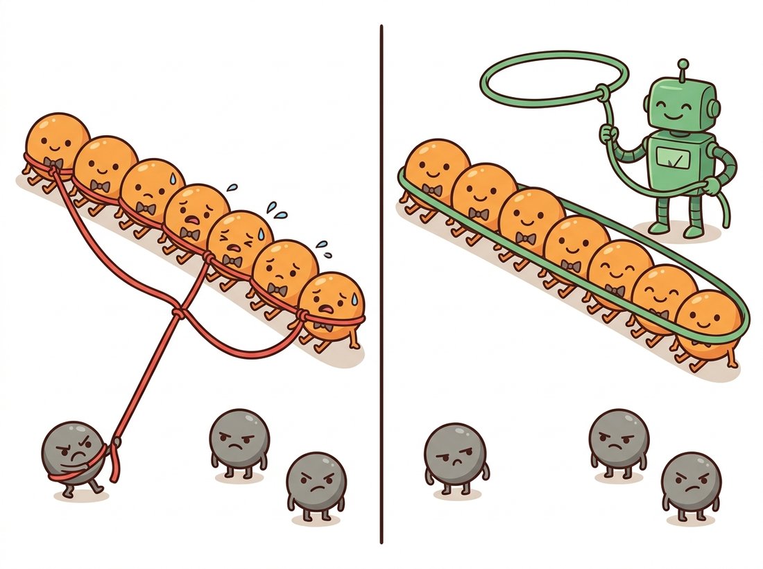
RANSAC (Random Sample Consensus, Fischler and Bolles, 1981) abandons the idea of weighing all points and instead hunts for the largest subset that agrees on one model. The loop is almost embarrassingly simple. Repeat $N$ times: draw the minimal sample that determines the model (2 points for a line, 3 for a circle, 4 correspondences for the homographies of Chapter 5); fit the model to the sample exactly; count the inliers, points within a tolerance $\tau$ of the model. Keep the hypothesis with the most inliers, then refit precisely (TLS or an M-estimator) on its consensus set. Outliers cannot sabotage hypotheses they are not sampled into, and a hypothesis built from two honest points collects the whole honest population as supporters.

The number of iterations is not folklore; it is arithmetic. If the inlier fraction is $w$ and the minimal sample has $s$ points, one draw is all-inlier with probability $w^s$, so the number of iterations needed to see at least one clean draw with confidence $p$ is

$$ N \;=\; \frac{\ln(1 - p)}{\ln(1 - w^s)}. $$

For a line ($s = 2$) with half the points outliers ($w = 0.5$) and $p = 0.99$, $N = 17$: seventeen tries to fit a line through 50 percent garbage, which is why RANSAC feels like cheating the first time it works. The formula's sting is the exponent: for a fundamental matrix with $s = 8$ at $w = 0.5$, $N \approx 1{,}177$, and at $w = 0.3$ it explodes past 70,000, the reason Chapter 13 cares so much about minimal solvers and inlier-rate boosters. Figure 9.4.2 shows the consensus logic that makes the whole thing tick.

import numpy as np

def ransac_line(pts, n_iter=100, tol=2.0, seed=0):
    rng = np.random.default_rng(seed)
    best_inl = None
    for _ in range(n_iter):
        i, j = rng.choice(len(pts), size=2, replace=False)   # minimal sample
        p, q = pts[i], pts[j]
        d = q - p
        n = np.array([-d[1], d[0]]) / (np.hypot(*d) + 1e-12) # unit normal
        resid = np.abs((pts - p) @ n)                        # point-line dist
        inl = resid < tol
        if best_inl is None or inl.sum() > best_inl.sum():
            best_inl = inl
    # final polish: TLS on the consensus set only
    sel = pts[best_inl]
    c = sel - sel.mean(axis=0)
    _, eigvec = np.linalg.eigh(c.T @ c)
    return eigvec[:, -1], sel.mean(axis=0), best_inl

# same contaminated data as the cv2.fitLine demo above
direction, centroid, inl = ransac_line(pts)
print(f"inliers found: {inl.sum()}/{len(pts)}, "
      f"slope {direction[1] / direction[0]:+.3f}")
# Representative output:
# inliers found: 60/66, slope +0.501

5. Fitting Ellipses Directly Advanced

One conic deserves special mention because it appears whenever circles are photographed: perspective turns circles into ellipses, so pupils, drilled holes, plates, and the calibration dots of Chapter 12 all reach the fitter as ellipse data. The general conic $a x^2 + b x y + c y^2 + d x + e y + f = 0$ is linear in its six coefficients, but a naive least-squares solve happily returns hyperbolas and parabolas when the data is noisy or covers only an arc. Fitzgibbon, Pilu, and Fisher's 1999 method imposes the constraint $4ac - b^2 = 1$, which forces ellipse-ness algebraically, and the constrained problem collapses to a small generalized eigenvalue system: a closed-form, always-an-ellipse fit. That is the algorithm inside OpenCV:

import cv2
import numpy as np

mask = cv2.imread("pupil_mask.png", cv2.IMREAD_GRAYSCALE)  # binary blob
contours, _ = cv2.findContours(mask, cv2.RETR_EXTERNAL,
                               cv2.CHAIN_APPROX_NONE)
cnt = max(contours, key=cv2.contourArea)        # largest blob's boundary

(cx, cy), (minor, major), angle = cv2.fitEllipse(cnt)  # needs >= 5 points
print(f"center ({cx:.1f}, {cy:.1f}), axes {minor:.1f} x {major:.1f} px, "
      f"tilt {angle:.1f} deg")
# Representative output:
# center (212.4, 156.8), axes 38.2 x 51.6 px, tilt 14.3 deg

The same robustness caveats apply at this level too: cv2.fitEllipse is a least-squares method, so eyelash occlusions or specular bites on the contour call for the RANSAC wrapper (five points is the minimal ellipse sample) or for skimage.measure.EllipseModel inside skimage.measure.ransac, which composes exactly the two-step recipe this section has been building.