Worked Example: Lane-Marking Detection

"The lane was clearly marked for two hundred kilometers. Then it rained, the sun came back out, and I learned that I had spent my entire career detecting dry weather."

A Recently Humbled Lane Detector

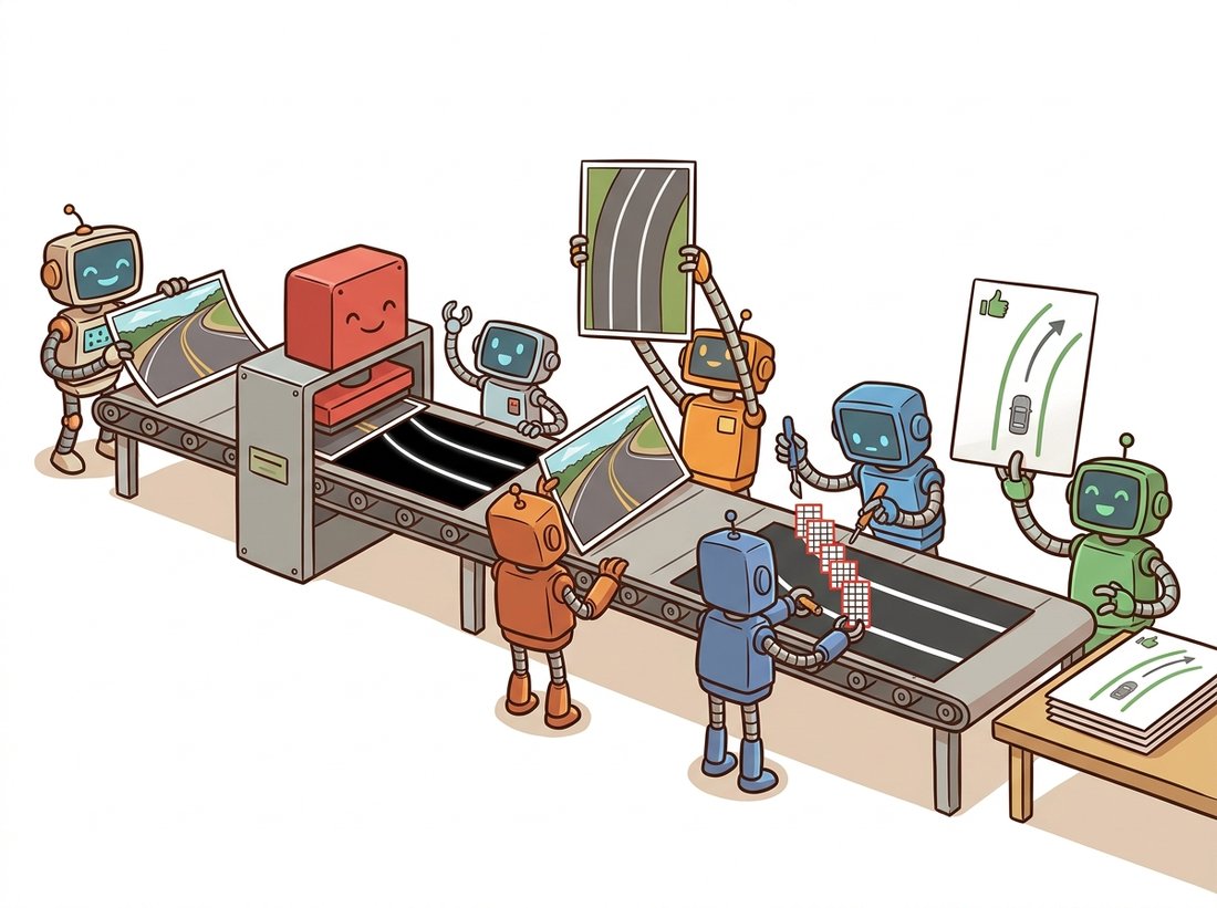
The previous section closed the chapter's toolbox: we can detect structure by voting and measure it by fitting, even when most of the evidence is contaminated. What remains is the engineering question: do the pieces compose into a system that does something useful? Lane-marking detection is the canonical test because it needs every piece at once, and because its failure modes, catalogued deliberately at the end, are the best argument anyone has ever made for Part III.

1. The Assignment: From Dashcam Frame to Steering Geometry Beginner

The input is a forward-facing camera frame, say $1280 \times 720$ pixels at 30 frames per second. The output a lane-keeping controller wants is compact: the lane's two boundary markings as curves in road coordinates, the radius of curvature of the lane ahead in meters, and the car's lateral offset from the lane center. Note what is being asked: not "which pixels are paint" but "where is the lane, as a measurable curve in the world." That is the chapter's pixels-to-geometry trajectory, pushed one step further into physical units.

Figure 9.5.1 shows the pipeline. One precondition is handled offstage: the frame must be undistorted, because consumer lenses bend straight lane lines into gentle arcs near the image border, and a curve fitter cannot tell optical bending from road curvature. Chapter 12 builds the calibration that removes lens distortion; here we assume it has been applied. Everything else in the figure is this chapter, plus one homography from Chapter 5.

A word on budget: at 30 frames per second the pipeline has 33 milliseconds per frame, shared with everything else the vehicle computer does. Every operation below is a thresholded filter, one warp, a histogram, or a small linear solve; on one CPU core the whole pipeline runs in a few milliseconds, which is why Section 9.1 made a point of the libraries running their kernels separably in optimized C. This arithmetic is much of why classical lane detection shipped.

2. Stage 1: Thresholding for Evidence Intermediate

The first stage converts the frame into a binary mask: 1 where a pixel plausibly belongs to lane paint, 0 elsewhere. We combine two independent kinds of evidence, because each one alone has a famous failure mode.

Gradient evidence. Lane markings in a forward-facing camera run roughly toward the vanishing point, so they are close to vertical in the image and their intensity changes are close to horizontal. An $x$-direction Sobel filter, exactly the instrument calibrated in Section 9.1, responds to lane edges while staying quiet on horizontal structure like shadow lines cast across the road. But recall the ridge profile from Section 9.1: a paint stripe is a thin bright line, so the gradient fires on both flanks and returns every marking as a double line. This is the annoyance Section 9.1 promised we would deal with directly; the fix is the second channel.

Color evidence. Lane paint is engineered to be visible, which in color terms means saturated white or yellow. The S channel of the HLS representation from Chapter 1 captures exactly this: paint stays high-saturation as overall brightness drops into shade, where raw RGB thresholds collapse. A fixed threshold on S, chosen with the histogram-reading skills of Chapter 2, lights up the body of each stripe, not just its flanks, so the union of the two channels turns every marking into one solid blob and dissolves the double-line problem; a single morphological opening from Chapter 6 then deletes the speckles both channels produce. The function below implements the whole stage.

import cv2
import numpy as np

def lane_evidence(bgr):
    """Binary mask of likely lane-paint pixels: gradient OR color."""
    gray = cv2.cvtColor(bgr, cv2.COLOR_BGR2GRAY)
    sx = cv2.Sobel(gray, cv2.CV_64F, 1, 0, ksize=3)     # x-gradient only
    sx = np.uint8(255 * np.abs(sx) / (np.abs(sx).max() + 1e-12))
    grad = sx >= 35                       # fires on both flanks of a stripe
    hls = cv2.cvtColor(bgr, cv2.COLOR_BGR2HLS)
    color = hls[:, :, 2] >= 120           # S channel: paint stays saturated
    mask = (grad | color).astype(np.uint8) * 255
    kernel = np.ones((3, 3), np.uint8)    # one opening pass kills speckle
    return cv2.morphologyEx(mask, cv2.MORPH_OPEN, kernel)

frame = cv2.imread("highway_frame.jpg")   # 1280 x 720, lens-undistorted
mask = lane_evidence(frame)
print(f"evidence pixels: {(mask > 0).mean():.1%} of the frame")
# Representative output:
# evidence pixels: 3.4% of the frame

Notice what we did not use: the full Canny detector of Section 9.2. Canny's non-maximum suppression thins edges to one pixel, which is ideal when edges are the product but counterproductive here, where we want fat blobs of paint pixels for the histogram search to count. Choosing which tool a stage actually needs, rather than the most sophisticated tool available, is most of pipeline engineering.

3. Stage 2: The Bird's-Eye Warp Intermediate

In the camera view, perspective entangles everything: parallel lane lines converge, lane width shrinks with distance, and a constant-curvature arc projects to a curve whose shape depends on where it sits in the frame. Fitting and measuring in that view means undoing perspective inside the model. The classical move is to undo it in the image instead: warp the road plane to a synthetic overhead view, after which lane lines are near-vertical and parallel, lane width is constant in pixels, and a quadratic $x = Ay^2 + By + C$ is an excellent local model of real road geometry (highways are built from clothoid arcs, which a quadratic tracks closely over a 30 meter window).

The warp is a planar homography, exactly the $3 \times 3$ machinery built in Chapter 5: the road is (assumed) flat, so four point correspondences determine the mapping. Calibration is a one-time manual act: on a frame where the road is known to be straight, mark a trapezoid whose sides lie on the two lane lines, and declare that it should map to a rectangle. The code below performs the warp; Figure 9.5.2 (in the next stage) shows it visually.

h, w = mask.shape
# source trapezoid: marked once on a straight-road frame, reused forever
src = np.float32([[w * 0.43, h * 0.65], [w * 0.57, h * 0.65],
                  [w * 0.90, h * 0.96], [w * 0.10, h * 0.96]])
dst = np.float32([[w * 0.25, 0], [w * 0.75, 0],
                  [w * 0.75, h], [w * 0.25, h]])
M    = cv2.getPerspectiveTransform(src, dst)   # 3x3 homography
Minv = cv2.getPerspectiveTransform(dst, src)   # for painting results back
birds = cv2.warpPerspective(mask, M, (w, h),
                            flags=cv2.INTER_NEAREST)  # keep mask binary

Two warnings. First, the flat-road assumption is real: crests, dips, and braking pitch tilt the true road plane away from the calibrated one, and the warp answers by bending straight lanes into phantom curves; production systems estimate pitch online. Second, the warp resamples aggressively near the top of the trapezoid, one source pixel smearing across many destination pixels, which is why we threshold before warping rather than after, a choice Exercise 9.5.1 asks you to defend.

4. Stage 3: Sliding-Window Search Intermediate

The warped mask contains lane blobs plus clutter: shadow fragments, asphalt seams, the occasional vehicle. Which evidence pixels belong to the left marking, which to the right, and which to neither? The classical answer starts with a wonderfully cheap idea: sum the mask's columns over the bottom half of the image. A near-vertical marking piles its pixels into a narrow range of columns, so the histogram shows two dominant peaks, and the peaks are the lanes' base positions at the bumper. From each base a stack of fixed-size windows climbs the image, each window recentering on the mean $x$ of the pixels it captures, so the stack tracks the marking as it curves, as Figure 9.5.2 illustrates.

The implementation below returns the raw pixel coordinates assigned to each marking, ready for fitting. It is deliberately plain NumPy: one histogram, one nonzero, and a short loop over windows.

def sliding_window_search(birds, n_windows=9, margin=80, minpix=50):
    """Collect lane pixels by climbing windows from two histogram peaks."""
    hist = birds[birds.shape[0] // 2:, :].sum(axis=0)   # bottom-half votes
    mid = hist.shape[0] // 2
    bases = [int(np.argmax(hist[:mid])), int(np.argmax(hist[mid:])) + mid]
    nz_y, nz_x = birds.nonzero()                        # all evidence pixels
    win_h = birds.shape[0] // n_windows
    keep = [[], []]                                     # left, right masks
    for k in range(n_windows):
        y_hi = birds.shape[0] - k * win_h               # window bottom
        y_lo = y_hi - win_h                             # window top
        for side, x0 in enumerate(bases):
            sel = ((nz_y >= y_lo) & (nz_y < y_hi) &
                   (np.abs(nz_x - x0) < margin))
            keep[side].append(sel)
            if sel.sum() > minpix:                      # recenter on the mean
                bases[side] = int(nz_x[sel].mean())
    out = []
    for side in (0, 1):
        sel = np.logical_or.reduce(keep[side])
        out.append((nz_x[sel], nz_y[sel]))
    return out                                          # [(xl, yl), (xr, yr)]

The minpix gate matters more than it looks: a window over a gap in a dashed marking catches almost nothing, and recentering on three noise pixels would fling the stack sideways; by refusing to recenter on thin evidence, the stack coasts straight through dashes, the correct prior for road paint. On video there is a further shortcut: after a good fit, the next frame skips the histogram and windows and harvests evidence pixels within a margin of the previous polynomial. Exercise 9.5.2 builds that fast path and the sanity gates that decide when to fall back to the full search.

5. Stage 4: Polynomials, Curvature, and Meters Advanced

Now the measurement step. We fit each marking with the quadratic that Section 9.4 promised, in the lane-friendly orientation $x = Ay^2 + By + C$: $x$ as a function of $y$, because the markings are near-vertical and a $y$-on-$x$ fit would hit exactly the steep-line pathology that Section 9.4 dissected. Orienting the model along the data is the cheapest robustness trick in the entire pipeline.

The fit happens twice: once in pixel units for drawing the overlay, and once in metric units for the controller. The unit conversion is a calibration fact about the warp: our destination rectangle places the lane edges $0.5\,w = 640$ pixels apart, and a standard highway lane is $3.7$ meters wide, so one warped pixel is $3.7/640$ meters in $x$; the trapezoid was marked to cover roughly 30 meters of road, so one pixel is $30/720$ meters in $y$. With metric coefficients in hand, the radius of curvature of $x(y)$ at the bumper line $y_0$ is the standard formula from calculus:

$$ R \;=\; \frac{\bigl(1 + (2Ay_0 + B)^2\bigr)^{3/2}}{\lvert 2A \rvert}, $$

and the lateral offset is the difference between the image center (where the camera, and approximately the car, sits) and the midpoint of the two fitted curves at the bumper, scaled to meters. The code below completes the pipeline.

XM = 3.7 / 640    # meters per warped pixel in x: lane width 3.7 m = 640 px
YM = 30.0 / 720   # meters per warped pixel in y: warp covers ~30 m of road

(xl, yl), (xr, yr) = sliding_window_search(birds)
left_px  = np.polyfit(yl, xl, 2)          # x = A y^2 + B y + C, in pixels
right_px = np.polyfit(yr, xr, 2)
left_m   = np.polyfit(yl * YM, xl * XM, 2)        # same fit, metric units

A, B, _ = left_m
y_car = (h - 1) * YM                       # evaluate at the bumper line
radius = (1 + (2 * A * y_car + B) ** 2) ** 1.5 / abs(2 * A)

lane_mid = (np.polyval(left_px, h - 1) + np.polyval(right_px, h - 1)) / 2
offset = (w / 2 - lane_mid) * XM           # + means car is right of center
print(f"radius of curvature {radius:7.0f} m   lateral offset {offset:+.2f} m")
# Representative output:
# radius of curvature     886 m   lateral offset -0.12 m

On a clean frame, plain least squares is the right fitter, because the sliding windows have already done the robustness work: they are a membership filter, the two-step recipe of Section 9.4 wearing different clothes. On a bad frame the corridor itself can be captured: Section 9.4 warned that most thresholded pixels can belong to shadows and asphalt texture rather than paint, and a window stack can lock onto a shadow band running beside the marking. Production pipelines therefore add defenses: sanity gates that reject a frame whose two fits are not roughly parallel, whose implied lane width is wrong at any of three heights, or whose left and right curvatures disagree wildly; temporal smoothing that coasts on the last good fit through rejected frames, a job done properly by the Kalman filters of Chapter 15; and, on the worst frames, a RANSAC fit over the window centroids, exactly as built in Section 9.4.

6. When It Breaks, and What Replaced It Intermediate

Run this pipeline on a sunny highway and it looks unreasonably good. Run it on the full diversity of real driving and its failure taxonomy emerges clearly, because each failure is a violated assumption you can name:

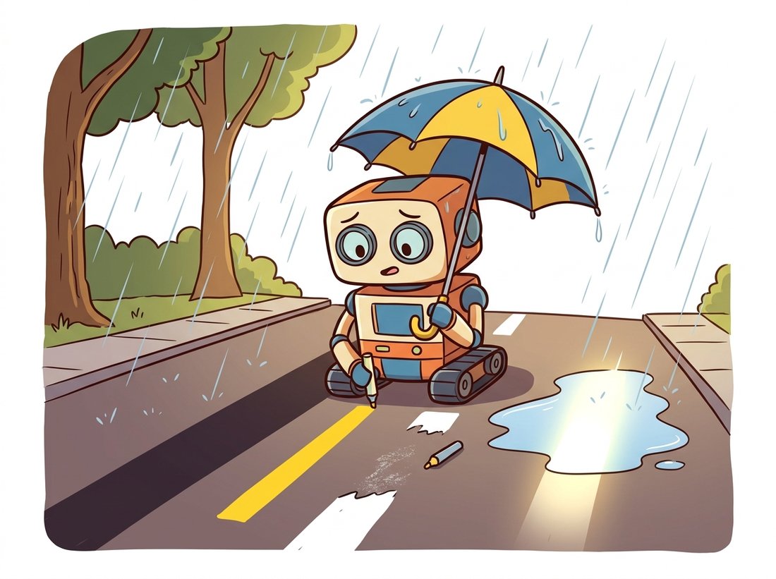
• Shadows and glare violate the threshold stage: a tree line casts high-contrast edges that out-vote faded paint, and wet asphalt mirrors the sky into the saturation channel.
• Worn or absent paint violates the evidence assumption outright; no threshold recovers markings that are not there, while human drivers infer the lane from curbs, traffic, and habit.
• Hills and braking pitch violate the flat-road homography, bending straight lanes into phantom curves.
• Lane changes and merges violate the two-peak histogram model precisely when geometry matters most.
• Unusual markings (double yellows, botts' dots, temporary construction lines painted over old ones) violate the one-stripe-per-side prior.

The CULane benchmark formalizes exactly this taxonomy, with test categories for shadow, glare, night, no-line, and curve frames; classical pipelines score respectably on the clean categories and collapse on the rest. That gap is the empirical case for learning the evidence rather than hand-coding it: the convolutional networks of Chapter 19 learn their own thresholds from data (their first layers rediscover oriented gradient filters on their own), and the segmentation machinery of Chapter 24 replaces threshold-and-search with a per-pixel classifier trained on tens of thousands of annotated frames. What deep models did not discard is the geometry: outputs are still fit with curve models and evaluated in curvature and lateral offset. The vocabulary this pipeline defined became the field's evaluation language.

This closes the chapter's arc: we began with a philosophical question (what is an edge?) and ended with a machine that converts two million pixels into a curvature radius a controller can steer by, exercising gradients as instruments, voting as detection, consensus as robustness, and fitting as measurement along the way. The next chapter changes strategy: instead of long anonymous contours grouped by geometric priors, Chapter 10 finds compact, recognizable points and gives each a fingerprint descriptor, the move that makes two photographs of the same scene comparable; the RANSAC you now know travels there immediately.