Epipolar Geometry: The Geometry of Two Views

"I cannot tell you exactly where your point went in the other photograph. But I can tell you the one line it is hiding on, which narrows things down from a million suspects to about a thousand. You're welcome."

A Helpfully Restrictive Epipolar Line

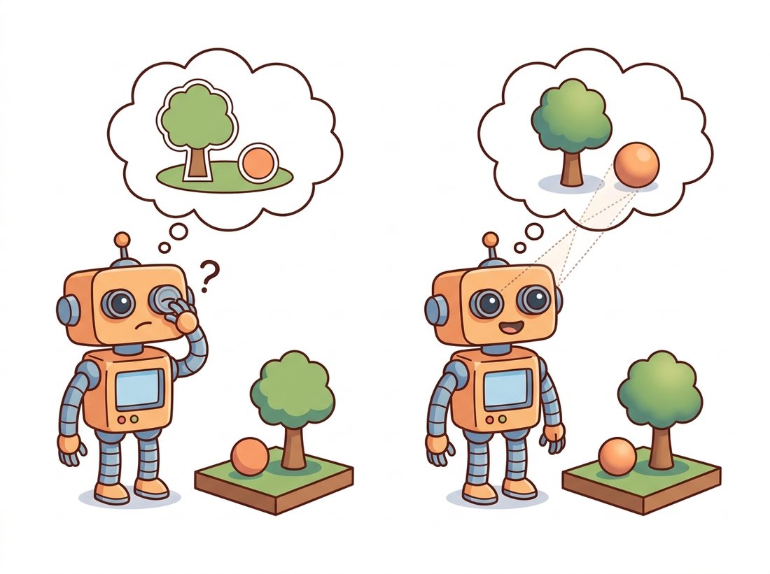
Chapter 12 left us with a precise account of what one camera does: it projects each 3D point along a ray through the optical center onto the image plane, and the intrinsic matrix $K$ tells us exactly which pixel that ray hits. It also left us with a loss we could not repair. Every point on a given ray, whether one meter away or one kilometer, lands on the same pixel. Depth is not hidden in a single image; it is absent. This section begins the repair, and the tool is almost embarrassingly simple: take a second photograph from somewhere else.

1. What a Second View Knows Beginner

Consider a point $\mathbf{x}_L$ in the left image. From the left camera's perspective, the 3D point $\mathbf{X}$ that produced it could be anywhere along the viewing ray from the left optical center $\mathbf{C}_L$ through $\mathbf{x}_L$. One image cannot say more. Now ask what the right camera sees. It observes that same ray from the side, and a ray, viewed from anywhere not on it, projects to a line. So whatever depth $\mathbf{X}$ actually has, its image in the right view must fall on the projection of the left ray: a single line in the right image, called the epipolar line.

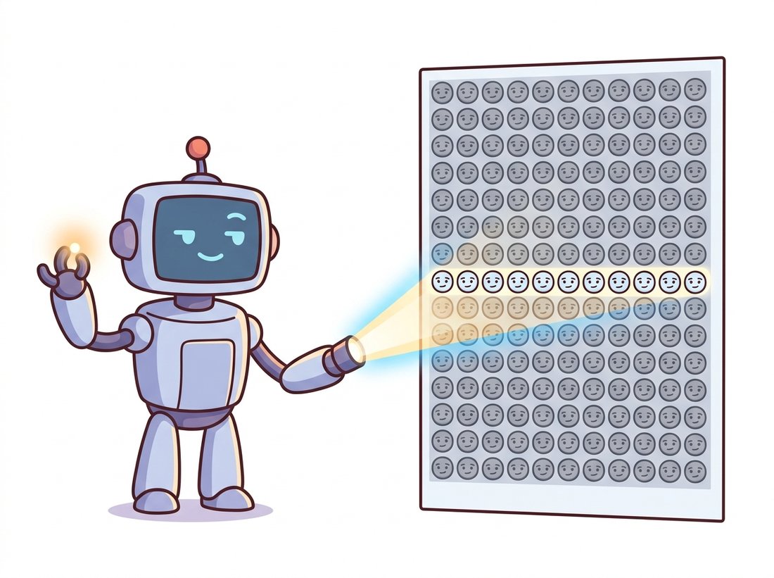
This deserves a moment of appreciation. We have not measured anything yet, not matched a single descriptor, and already the geometry has handed us an enormous gift: the correspondence problem of Chapter 10, which searched a whole 2D image for each match, has become a 1D search along a known line. For a $1000 \times 1000$ image, that is a thousandfold reduction in candidates before any pixel is compared.

2. The Epipolar Vocabulary Intermediate

The full structure becomes visible when you draw both cameras and one 3D point, as in Figure 13.1.1. Three points define the picture: the two optical centers $\mathbf{C}_L$, $\mathbf{C}_R$, and the scene point $\mathbf{X}$. Together they span a plane, the epipolar plane. Everything else is intersections of that plane with the two image planes.

Working through Figure 13.1.1 gives the complete glossary. The baseline is the segment joining the two optical centers; its length, also called the baseline, will set the depth precision of stereo in Section 13.5. The epipoles $\mathbf{e}_L$ and $\mathbf{e}_R$ are where the baseline pierces each image plane: the epipole in the left image is literally the photograph of the right camera's center, and vice versa. The epipolar plane intersects each image plane in an epipolar line, and since both $\mathbf{x}_L$ and $\mathbf{x}_R$ are images of a point on that plane, each must lie on its line.

Now let $\mathbf{X}$ slide to different depths along the left viewing ray. The epipolar plane does not change (the ray lies inside it), so the right epipolar line does not change either; the match $\mathbf{x}_R$ just slides along it. But pick a different pixel $\mathbf{x}_L$, and the plane rotates about the baseline like a page turning on its spine, sweeping out a new pair of epipolar lines. Two consequences follow immediately, and both are worth committing to memory:

• Every epipolar line passes through the epipole. The baseline lies in every epipolar plane, so its piercing points, the epipoles, lie on every epipolar line. The family of epipolar lines is a pencil of lines radiating from the epipole.
• Epipolar lines come in mated pairs. One plane cuts both images, so each epipolar line in the left image has exactly one partner in the right image, and matches can only happen between partners.

3. From Geometry to a Usable Test Intermediate

The constraint has a compact verbal form: corresponding points lie on corresponding epipolar lines. To make it computational we need a function that, given a point in one image, produces the epipolar line in the other. Section 13.2 will show that this function is linear in homogeneous coordinates: a single $3 \times 3$ matrix $F$, the fundamental matrix, maps a left point to a right line, $\boldsymbol{\ell}_R = F \mathbf{x}_L$, and the constraint becomes the elegant scalar equation $\mathbf{x}_R^\top F \mathbf{x}_L = 0$. For this section we treat $F$ as a black box that OpenCV can estimate from matched keypoints, and concentrate on what the resulting lines look like and how to use them.

A line in homogeneous coordinates is a 3-vector $\boldsymbol{\ell} = (a, b, c)^\top$ representing $ax + by + c = 0$, a representation introduced with projective transforms in Chapter 5. The perpendicular distance from a pixel $(x, y)$ to that line is

$$ d\big((x,y),\, \boldsymbol{\ell}\big) \;=\; \frac{|ax + by + c|}{\sqrt{a^2 + b^2}}, $$

and this distance is the workhorse test of two-view geometry: a candidate correspondence is epipolar-consistent if each point sits within a pixel or two of its partner's epipolar line. The code below runs the full pipeline on a real pair: detect and match SIFT keypoints exactly as in Chapter 10, estimate $F$ robustly, then compute and draw the epipolar lines for a handful of inlier matches.

import cv2
import numpy as np

imgL = cv2.imread("left.jpg", cv2.IMREAD_GRAYSCALE)
imgR = cv2.imread("right.jpg", cv2.IMREAD_GRAYSCALE)

# 1. Correspondences, exactly as in Chapter 10: SIFT + ratio test
sift = cv2.SIFT_create()
kpL, desL = sift.detectAndCompute(imgL, None)
kpR, desR = sift.detectAndCompute(imgR, None)
knn = cv2.BFMatcher(cv2.NORM_L2).knnMatch(desL, desR, k=2)
good = [m for m, n in knn if m.distance < 0.75 * n.distance]
ptsL = np.float32([kpL[m.queryIdx].pt for m in good])
ptsR = np.float32([kpR[m.trainIdx].pt for m in good])

# 2. Robust fundamental matrix (MAGSAC++ flavor of RANSAC)
F, inlier_mask = cv2.findFundamentalMat(ptsL, ptsR,
                                        cv2.USAC_MAGSAC, 1.0, 0.999)
inl = inlier_mask.ravel().astype(bool)
print(f"{inl.sum()} / {len(good)} matches are epipolar-consistent")
# 487 / 612 matches are epipolar-consistent

# 3. Epipolar lines in the LEFT image for right-image inlier points
#    (whichImage=2 means the points live in image 2, the right one)
linesL = cv2.computeCorrespondEpilines(ptsR[inl], 2, F).reshape(-1, 3)
a, b, c = linesL[0]
x0, x1 = 0, imgL.shape[1]
y0, y1 = int(-c / b), int(-(c + a * x1) / b)   # line endpoints at image borders
vis = cv2.cvtColor(imgL, cv2.COLOR_GRAY2BGR)
cv2.line(vis, (x0, y0), (x1, y1), (0, 0, 255), 1)
cv2.circle(vis, tuple(ptsL[inl][0].astype(int)), 5, (0, 255, 0), -1)
cv2.imwrite("epiline_left.png", vis)

Run this on any pair of photos of a static scene and inspect the output image: the red line should pass through the green point, typically within a pixel. Repeating the drawing for ten matches produces ten lines that all radiate from a common (often off-image) point, the epipole, exactly as the pencil-of-lines picture predicts. When the lines do not converge, or the points sit far off their lines, something upstream is wrong: bad matches that RANSAC failed to reject, a moving object dominating the correspondences, or a degenerate configuration of the kind Section 13.2 and Section 13.3 dissect.

4. Special Configurations Worth Recognizing Intermediate

Two camera arrangements produce epipolar geometry so distinctive that you should recognize them on sight, because entire system designs are built around each.

Side-by-side cameras (the stereo configuration). When the two cameras are related by a pure horizontal translation with parallel optical axes, the baseline is parallel to both image planes and never pierces them: the epipoles move to infinity. The pencil of epipolar lines, all forced through a point at horizontal infinity, becomes a family of parallel horizontal lines, and corresponding points share the same row. This is the dream configuration for dense matching, and Section 13.4 exists because of it: rectification is nothing but warping an arbitrary pair until its epipolar geometry looks like this.

Forward motion. When the camera translates along its own optical axis (a car driving forward, a drone descending), the baseline pierces both image planes at the principal point: both epipoles sit in the middle of the image, and epipolar lines radiate outward from the center like spokes. Matches slide outward along the spokes as the camera advances. This radial pattern is the focus of expansion that Chapter 15 revisits with optical flow, and it is the hardest case for stereo matching: near the epipole, the epipolar "line" segment available for matching shrinks to nearly nothing, and depth becomes unobservable along the motion axis.

5. Where the Constraint Comes From, and Where It Breaks Advanced

It is worth being precise about the assumptions, because every failure of two-view geometry in practice traces back to one of them. The epipolar constraint requires exactly three things: a static scene point (so that both cameras photograph the same $\mathbf{X}$), two distinct optical centers (so that a plane, not a line, is spanned), and cameras that behave like pinholes (so that projection is along straight rays, the assumption Chapter 12 spent a whole section repairing with distortion correction; always undistort before doing epipolar geometry).

Each assumption fails in an instructive way. A moving object violates the static-scene premise: its matches satisfy a different epipolar geometry (one induced by the object's motion composed with the camera's), which is why points on a passing truck show up as outliers to the road's fundamental matrix, and why motion segmentation can be built from exactly this observation, a thread picked up in Chapter 15. Coincident optical centers (a camera rotating on a tripod) collapse the epipolar plane: with no baseline there are no epipoles, no epipolar lines, and no depth, but in exchange the two views become related by a homography, which is precisely the subject of Section 13.3. And uncorrected lens distortion bends the straight rays, turning epipolar lines into epipolar curves that a $3 \times 3$ matrix cannot represent; the symptom is a fundamental-matrix fit whose inliers cluster in the image center while the corners misbehave.

6. What Comes Next Beginner

This section built the geometry with pictures and one black box: the matrix that maps points to lines. Everything ahead in the chapter unpacks or exploits it. Section 13.2 derives that matrix in two flavors (essential for calibrated cameras, fundamental for uncalibrated ones), shows how to estimate it from eight matches, and extracts the relative camera pose hiding inside it. Section 13.4 warps image pairs into the side-by-side configuration where epipolar lines are scanlines and matches densely. And Section 13.6 intersects the rays the constraint has been guarding all along, turning matched pixels into measured 3D points, the currency in which Chapter 14 and the neural 3D methods of Chapter 27 trade.