Homographies & Panorama Stitching

"My worldview is simple: everything is flat, or I never moved. People call that reductive. I call it nine numbers, and my panoramas look great."

A Homography With a Conveniently Flat Worldview

The previous section flagged planar scenes and pure rotation as degeneracies that break fundamental-matrix estimation. This section flips the perspective: those "degenerate" cases are not broken geometry but stronger geometry. When the scene is a plane, or the camera only rotates, the second view is fully determined by the first, point for point, and the map between them is the projective transform you met as a pure warping tool in Chapter 5. What Chapter 5 treated as an arbitrary $3 \times 3$ warp now acquires its physics.

1. Two Roads to a Point-to-Point Map Intermediate

Why does the general two-view relation stop at point-to-line? Because depth is free: a pixel in the left image could be any point on its ray, and different depths land at different places along the right epipolar line. A homography arises whenever something removes that freedom.

Road one: the scene is a plane. If every observed point lies on a single 3D plane with unit normal $\mathbf{n}$ at distance $d$ from the left camera, then the ray of each left pixel intersects the plane at exactly one point; depth is no longer free but determined. Pushing that intersection through the right camera's projection gives a closed-form pixel-to-pixel map,

$$ H \;=\; K_R \left( R \;-\; \frac{\mathbf{t}\, \mathbf{n}^\top}{d} \right) K_L^{-1}, $$

the plane-induced homography. Facades, floors, whiteboards, documents, sports fields, and (from a drone at altitude) entire landscapes qualify as planes, which is why this case carries so much industrial weight: every document scanner and every broadcast-sports overlay is this equation at work.

Road two: the camera never translates. Set $\mathbf{t} = 0$ and the plane drops out of the formula entirely: $H = K_R \, R \, K_L^{-1}$. With no baseline, all viewing rays of both views pass through the same optical center; the two images are two croppings of the same bundle of rays, and any scene, at any depth, maps point-to-point. This is the panorama case: rotate on a tripod (or hand-hold and stay close to pure rotation) and the views stitch exactly, no matter how three-dimensional the world is. The price was paid in Section 13.1: zero baseline means zero depth information. A panorama is geometrically gorgeous and metrically empty.

2. Estimating H: The Direct Linear Transform Advanced

A homography acts on homogeneous points as $\mathbf{x}' \sim H\mathbf{x}$, where $\sim$ means equality up to scale. Cross-multiplying away the unknown scale, each correspondence yields two independent linear equations in the nine entries of $H$, so four matches in general position determine it (eight equations, nine unknowns, one scale). With more matches, the same SVD null-space recipe as the eight-point algorithm applies, and the same Hartley normalization is just as mandatory; the construction is called the Direct Linear Transform (DLT). The implementation is fifteen lines:

import cv2
import numpy as np

def dlt_homography(src, dst):
    """H mapping src -> dst (each Nx2), via the normalized DLT."""
    (s, Ts), (d, Td) = normalize_points(src), normalize_points(dst)
    rows = []
    for (x, y, _), (u, v, _) in zip(s, d):
        # two equations per match from x' x (H x) = 0
        rows.append([-x, -y, -1,  0,  0,  0, u * x, u * y, u])
        rows.append([ 0,  0,  0, -x, -y, -1, v * x, v * y, v])
    A = np.asarray(rows)
    _, _, Vt = np.linalg.svd(A)
    H = Vt[-1].reshape(3, 3)
    H = np.linalg.inv(Td) @ H @ Ts      # undo normalization
    return H / H[2, 2]

H_ours = dlt_homography(ptsL[inl], ptsR[inl])
H_cv, _ = cv2.findHomography(ptsL[inl], ptsR[inl], 0)  # 0 = plain least squares
print(np.abs(H_ours - H_cv).max())      # ~1e-6: same answer

As with $F$, real matches need a robust wrapper: cv2.findHomography(src, dst, cv2.USAC_MAGSAC, 3.0) runs the DLT on minimal four-point samples inside MAGSAC++, scoring inliers by reprojection distance $\lVert \mathbf{x}' - \pi(H\mathbf{x}) \rVert$, where $\pi$ is the dehomogenization. This is the very call that Chapter 10 used as its RANSAC showcase; now you know what the model means physically and when it is the right one to fit.

3. The Panorama Pipeline Intermediate

Stitching two photographs taken from one viewpoint is now a four-stage assembly of parts you already own, summarized in Figure 13.3.1: correspondences from Chapter 10, a robust homography from this section, a warp from Chapter 5, and a blend to hide the seam.

The code below stitches two images along Figure 13.3.1's path. The only genuinely new engineering is canvas management: the warped image B may land partly at negative coordinates, so the homography is composed with a translation that shifts everything into view.

import cv2
import numpy as np

imgA = cv2.imread("pano_left.jpg")    # taken rotating on one spot
imgB = cv2.imread("pano_right.jpg")

# 1-2. Match and fit H mapping B's pixels into A's frame
sift = cv2.SIFT_create()
kA, dA = sift.detectAndCompute(imgA, None)
kB, dB = sift.detectAndCompute(imgB, None)
knn = cv2.BFMatcher(cv2.NORM_L2).knnMatch(dB, dA, k=2)
good = [m for m, n in knn if m.distance < 0.75 * n.distance]
src = np.float32([kB[m.queryIdx].pt for m in good])
dst = np.float32([kA[m.trainIdx].pt for m in good])
H, mask = cv2.findHomography(src, dst, cv2.USAC_MAGSAC, 3.0)

# 3. Canvas: warp B's corners to find the bounding box of the union
hA, wA = imgA.shape[:2]; hB, wB = imgB.shape[:2]
cornersB = np.float32([[0, 0], [wB, 0], [wB, hB], [0, hB]]).reshape(-1, 1, 2)
warped = cv2.perspectiveTransform(cornersB, H)
allpts = np.vstack([warped.reshape(-1, 2),
                    [[0, 0], [wA, 0], [wA, hA], [0, hA]]])
x0, y0 = np.floor(allpts.min(axis=0)).astype(int)
x1, y1 = np.ceil(allpts.max(axis=0)).astype(int)
shift = np.array([[1, 0, -x0], [0, 1, -y0], [0, 0, 1]], dtype=np.float64)

# 4. Warp B, paste A, feather the overlap
pano = cv2.warpPerspective(imgB, shift @ H, (x1 - x0, y1 - y0))
pano[-y0:hA - y0, -x0:wA - x0] = imgA      # hard paste; feathering below
cv2.imwrite("panorama.png", pano)
print(pano.shape, f"{int(mask.sum())} inliers")  # e.g. (1184, 2693, 3) 633 inliers

The hard paste in the last step leaves a visible seam wherever exposure differs between shots, and real stitchers blend instead. The classical answer is multi-band blending: decompose both images into the Laplacian pyramids of Chapter 4, blend low-frequency bands over wide regions (hiding exposure mismatch) and high-frequency bands over narrow ones (keeping edges crisp), then collapse the pyramid. Production stitchers add two more refinements worth knowing by name: gain compensation, a least-squares fix of per-image exposure before blending, and cylindrical or spherical projection for many-image panoramas, since chaining flat homographies across a wide field of view stretches the end images absurdly; projecting onto a cylinder first keeps the canvas bounded.

4. When Panoramas Fail: Parallax Intermediate

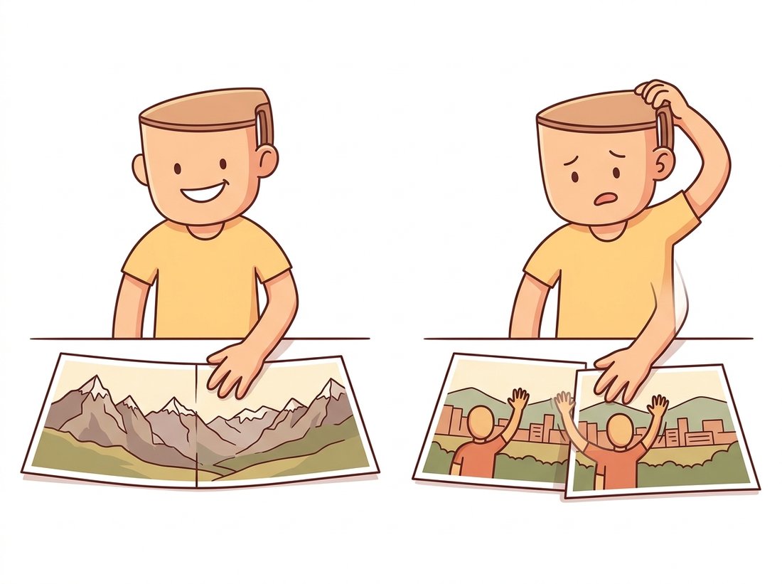
Every homography failure in the wild is the same failure: the capture violated one of the two roads of subsection 1. Hand-held panoramas are never pure rotation; the camera's optical center translates by a few centimeters between shots. For distant scenery the resulting parallax is a fraction of a pixel and invisible. For a subject two meters away, a 5 cm translation moves near and far objects differently by many pixels, no single homography fits both, and the stitcher produces the characteristic artifacts: ghosted double edges, severed railings, a friend's arm amputated at the seam. The fix hierarchy, in increasing order of effort: rotate about the lens's no-parallax point (tripod panorama heads exist for exactly this), stand farther back, keep seams away from near objects (seam-finding does this automatically), or admit the scene is 3D and graduate to the reconstruction machinery of the rest of this chapter.

5. Homographies Beyond Panoramas Beginner

The plane-induced road from subsection 1 powers a family of applications that have nothing to do with stitching, and recognizing them as "the same trick" is a mark of fluency. Document and whiteboard rectification fits $H$ from the four detected page corners to an upright rectangle and warps, the perspective correction of Chapter 5 now with automatically estimated parameters. Sports broadcasting maps the known geometry of the pitch to its image, so graphics can be painted onto the grass and player positions converted to field coordinates. Planar augmented reality tracks a poster or marker with a per-frame homography, and decomposing that homography (via cv2.decomposeHomographyMat, with $K$ known) recovers the camera's pose relative to the plane, the same pose-from-plane idea that rescued the drone mapper in Section 13.2's practical example. In every case the plane supplies the depth information a single view lacks, which is the entire lesson of this section in one sentence.