Attention & the Transformer Block, Vision Edition

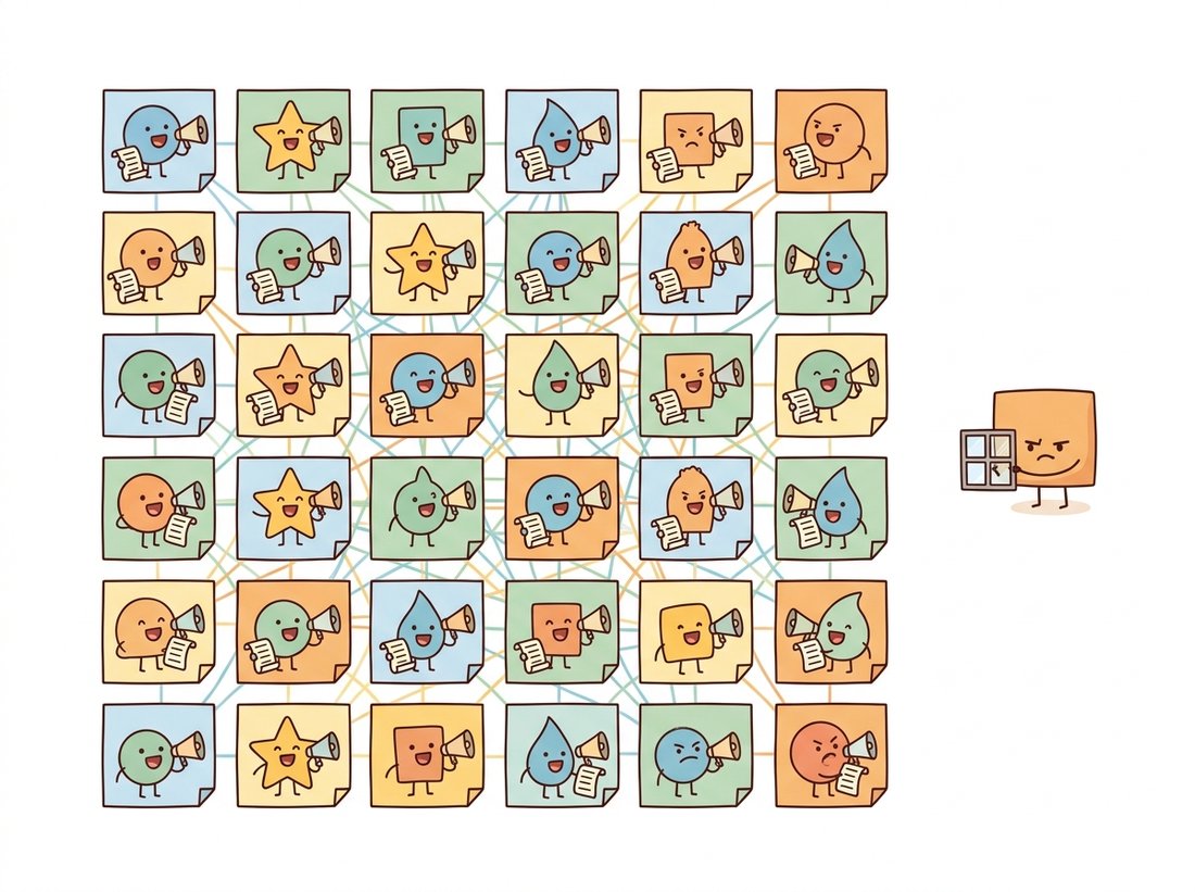
"A convolution asks each pixel, politely, what its neighbors are doing. Attention hands every patch a megaphone and a contact list. The room gets loud, but at least nobody is left out of the conversation."

An Attention Head That Reads the Whole Image at Once

In the previous chapters you built vision entirely out of convolutions. This section steps outside that world to construct the one new primitive the chapter needs. The transformer was introduced for language in 2017, but the operation at its core, self-attention, is not linguistic at all; it is a general way to let the elements of any set exchange information. Our plan is to derive it carefully on a generic sequence of tokens, implement each piece in PyTorch with the tools from Chapter 18, and only then, in Section 22.2, decide that the tokens are image patches. Keeping the derivation token-agnostic is deliberate: the same block will reappear for segmentation masks, video frames, and text conditioning later in the book, and you want to recognize it as one idea, not five.

1. From Dot Product to Attention Beginner

Start with the most basic question attention answers: given a sequence of $N$ vectors, how should each one update itself using information from the others? A reasonable answer is "average in the others, but weight each by how relevant it is to me." The dot product is our relevance measure. If two vectors point in similar directions, their dot product is large; if they are orthogonal, it is zero. So a first sketch of attention is: for token $i$, compute the dot product with every token $j$, normalize those scores into weights that sum to one, and form the output as the weighted sum of all tokens.

The transformer refines this in one important way. Rather than dotting the raw tokens against each other, it first projects each token through three separate learned linear maps to produce a query, a key, and a value. The query is "what am I looking for", the key is "what do I offer", and the value is "what I will actually contribute if you attend to me." The relevance of token $j$ to token $i$ is the dot product of $i$'s query with $j$'s key; the output for $i$ is the weighted sum of every token's value. Splitting one vector into these three roles lets the network learn to ask and answer different things, which a single shared representation cannot do.

Written compactly, with all queries stacked into a matrix $Q$, all keys into $K$, and all values into $V$, the entire operation is

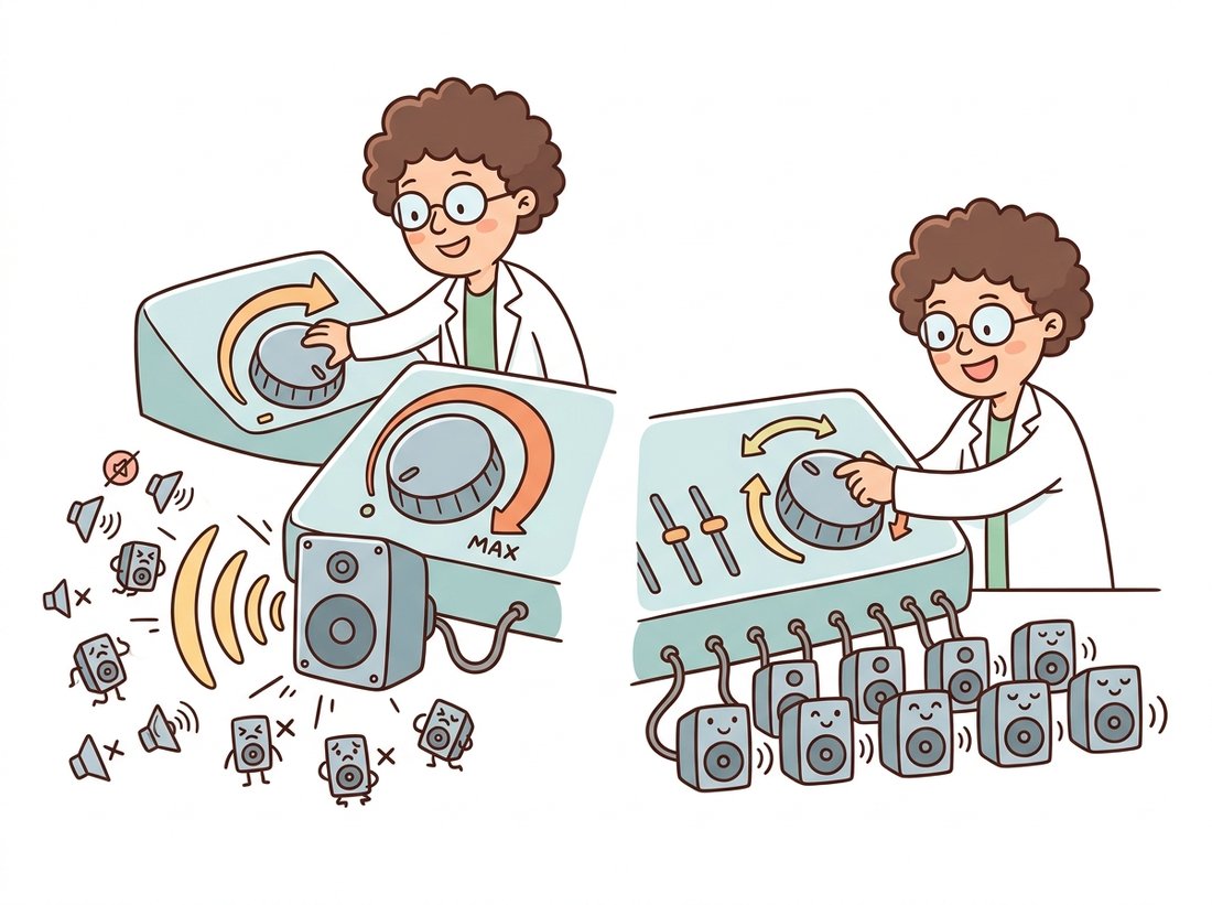
where $d_k$ is the dimension of the query and key vectors. The matrix $QK^\top$ holds every query-key dot product, one row per query; the softmax is applied along each row so the weights for one query sum to one; multiplying by $V$ forms the weighted sums. The division by $\sqrt{d_k}$ is the "scaled" in scaled dot-product attention, and it matters more than it looks. The dot product of two random $d_k$-dimensional vectors has variance proportional to $d_k$, so for large $d_k$ the scores grow large, the softmax saturates into a near one-hot spike, and its gradient nearly vanishes. Dividing by $\sqrt{d_k}$ holds the score variance near one and keeps the softmax in its responsive range.

The size of the effect is easy to underestimate. At the base ViT's head width $d_k = 64$, raw scores have a standard deviation of about $\sqrt{64} = 8$, so a typical query-key pair lands eight units apart, and $e^{8}$ is roughly $3000$ times $e^{0}$. One slightly-above-average key would therefore swallow almost the entire softmax row before training even begins. Dividing by $\sqrt{d_k} = 8$ shrinks that spread back to a standard deviation near one, where the softmax still listens to every patch. The whole stability of attention turns on that single factor of eight. Figure 22.1.1 traces these matrices through the computation, and the illustration below gives the intuition for that scale factor.

The code below implements exactly this formula on a batch of sequences. Read it against the figure: Q @ K.transpose is the score matrix, the scaling and softmax follow, and the final matmul with V produces the output.

# Scaled dot-product attention from the formula up: score every query
# against every key, normalize the scores with a softmax, then take the
# value-weighted sum. Passing one tensor as Q, K, and V gives self-attention.
import torch
import torch.nn.functional as F

def scaled_dot_product_attention(Q, K, V):
    """Q, K, V: (batch, seq_len, d_k). Returns (batch, seq_len, d_k) and weights."""
    d_k = Q.size(-1)
    scores = Q @ K.transpose(-2, -1) / d_k ** 0.5   # (batch, seq, seq)
    weights = F.softmax(scores, dim=-1)             # each query row sums to 1
    output = weights @ V                            # (batch, seq, d_k)
    return output, weights

# A toy batch: 1 sequence of 4 tokens, each of dimension 8.
torch.manual_seed(0)
X = torch.randn(1, 4, 8)
out, attn = scaled_dot_product_attention(X, X, X)  # self-attention: Q=K=V=X
print("output shape:", out.shape)       # output shape: torch.Size([1, 4, 8])
print("attention rows sum to:", attn.sum(-1))  # tensor([[1., 1., 1., 1.]])

2. Multi-Head Attention Intermediate

A single attention operation forces every token to summarize all of its relationships into one weighted average. That is limiting: a patch of an image might want to attend to texture in one sense and to global shape in another, and one softmax cannot represent both at once. Multi-head attention solves this by running several attention operations in parallel, each with its own learned query, key, and value projections, on lower-dimensional slices of the representation. Each head can specialize, one tracking local edges, another long-range layout, and their outputs are concatenated and passed through a final linear projection.

Concretely, with model dimension $d$ and $h$ heads, each head works in dimension $d_k = d / h$. Splitting this way keeps the total width fixed: $h$ heads of width $d/h$ recombine to width $d$, so multi-head attention costs essentially the same as one full-width head, it just spends that budget on several narrower views instead of one wide one. We project the input to $Q$, $K$, $V$ of full width $d$, reshape into $h$ heads of width $d_k$, run attention independently per head, concatenate back to width $d$, and apply an output projection $W_O$. The math is

Figure 22.1.2 traces this split-attend-concatenate path, and the implementation below packs all heads into single weight matrices for efficiency and reshapes to expose the head dimension, which is how every production library does it.

# Multi-head attention: project to Q, K, V with one fused matrix, split the
# width into independent heads so each can specialize, attend per head, then
# concatenate and re-project. The output shape matches the input so blocks stack.
import torch
import torch.nn as nn
import torch.nn.functional as F

class MultiHeadAttention(nn.Module):
    def __init__(self, dim, num_heads):
        super().__init__()
        assert dim % num_heads == 0, "dim must be divisible by num_heads"
        self.num_heads = num_heads
        self.d_k = dim // num_heads
        self.qkv = nn.Linear(dim, dim * 3)   # one matrix produces Q, K, V together
        self.proj = nn.Linear(dim, dim)      # output projection W_O

    def forward(self, x):
        B, N, D = x.shape
        qkv = self.qkv(x).reshape(B, N, 3, self.num_heads, self.d_k)
        qkv = qkv.permute(2, 0, 3, 1, 4)     # (3, B, heads, N, d_k)
        q, k, v = qkv[0], qkv[1], qkv[2]
        scores = q @ k.transpose(-2, -1) / self.d_k ** 0.5
        attn = F.softmax(scores, dim=-1)
        out = (attn @ v).transpose(1, 2).reshape(B, N, D)  # merge heads
        return self.proj(out)

mha = MultiHeadAttention(dim=64, num_heads=8)
x = torch.randn(2, 16, 64)               # batch 2, 16 tokens, dim 64
print("output shape:", mha(x).shape)     # output shape: torch.Size([2, 16, 64])

from torch.nn.functional import scaled_dot_product_attention as sdpa
# q, k, v shaped (B, heads, N, d_k); fused scale + softmax + matmul:
out = sdpa(q, k, v)   # no explicit scores tensor materialized in memory

3. The Transformer Block: Residuals, Norm, and an MLP Intermediate

Attention by itself is one operation; a transformer is a stack of blocks, and each block surrounds attention with three things you already know from Chapter 18 and Chapter 19: a residual connection, layer normalization, and a small feed-forward network (an MLP). The residual connection lets the input flow around each sub-layer, so gradients reach early layers cleanly and very deep stacks remain trainable, exactly the function residuals serve in the ResNet of Chapter 20. Layer normalization stabilizes the scale of activations across the feature dimension. The MLP, applied independently to each token, gives the block the non-linear capacity to transform what attention has gathered; transformers use GELU (the Gaussian Error Linear Unit) rather than the ReLU of Chapter 18, a smooth activation that gates each input by the probability a Gaussian sample falls below it, which trains more stably in this setting.

Modern transformers use the pre-norm arrangement: the normalization is applied before each sub-layer rather than after, which makes optimization far more forgiving and removes the need for the learning-rate warmup tricks that the original post-norm design required. A pre-norm block computes

Read that as: normalize, attend, add back; normalize, transform, add back. The residual stream (the running sum $x$) is never overwritten, only added to, which is why information from the patch embedding can reach the final layer directly. Figure 22.1.3 shows the two-sublayer block, and the code that follows assembles it from the multi-head attention of subsection 2.

# A pre-norm transformer block: LayerNorm then attention with a residual add,
# then LayerNorm then a 4x-expansion MLP with a residual add. Normalizing before
# each sub-layer keeps deep stacks trainable without learning-rate warmup.
import torch.nn as nn

class TransformerBlock(nn.Module):
    def __init__(self, dim, num_heads, mlp_ratio=4.0, dropout=0.0):
        super().__init__()
        self.norm1 = nn.LayerNorm(dim)
        self.attn = MultiHeadAttention(dim, num_heads)
        self.norm2 = nn.LayerNorm(dim)
        hidden = int(dim * mlp_ratio)
        self.mlp = nn.Sequential(
            nn.Linear(dim, hidden), nn.GELU(),   # GELU is the ViT-standard activation
            nn.Dropout(dropout),
            nn.Linear(hidden, dim), nn.Dropout(dropout),
        )

    def forward(self, x):
        x = x + self.attn(self.norm1(x))   # pre-norm attention sub-layer + residual
        x = x + self.mlp(self.norm2(x))    # pre-norm MLP sub-layer + residual
        return x

block = TransformerBlock(dim=64, num_heads=8)
import torch
print("block output:", block(torch.randn(2, 16, 64)).shape)  # torch.Size([2, 16, 64])

That block is the entire reusable engine of the chapter. Stack $L$ of these, feed them a sequence of token vectors, and you have a transformer encoder. The only thing left, the thing that turns this language-shaped machine into a vision model, is deciding what the tokens are and how to inject the spatial information that the permutation-invariant attention throws away. That is the subject of Section 22.2.

4. Why This Is Not a Convolution Advanced

It is worth making the contrast with the convolution precise, because the whole chapter turns on it. A convolution has three properties baked in by its very structure: locality (each output depends only on a small input neighborhood), weight sharing (the same kernel slides over every position, so the operation is translation-equivariant), and a fixed receptive field that grows only by stacking layers. These are inductive biases: assumptions about images that are true often enough to be enormously helpful, and that let a CNN learn from tens of thousands of images.

Self-attention discards all three. There is no locality: token $i$ attends to all $N$ tokens equally at the start, and the layer's effective neighborhood is the whole image from the very first block. There is weight sharing, but only of a different kind. The projection matrices are shared across positions, yet the attention pattern itself is not fixed; it is recomputed for every input. And the receptive field is global immediately, not grown over depth. A ViT therefore starts with almost no built-in knowledge that nearby pixels are related; it must learn that fact, if it is useful, from data. The cost is paid in two currencies. First, data: Section 22.3 is entirely about how to pay it. Second, compute: because every token attends to every other, the cost of self-attention is quadratic in the number of tokens.

For a $224 \times 224$ image cut into $16 \times 16$ patches, $N = 196$ tokens, and $N^2$ is manageable. Push to high-resolution dense prediction with thousands of tokens and the quadratic term dominates, which is precisely the problem the windowed attention of Section 22.4 exists to solve. The practical example below shows how this quadratic wall bites a real team.