ViT: Images as Sequences of Patches

"They handed me a sentence with no word order and asked me to translate it. So I stuck a little numbered sticker on every word. The stickers were the whole trick. Lose them and a cat becomes a bag of fur in random places."

A Positional Embedding That Refuses to Be Forgotten

In Section 22.1 we built a transformer encoder that operates on any sequence of token vectors, and we deliberately left the tokens abstract. Now we make them concrete. The reader who has spent four chapters thinking in feature maps may find the move jarring: we are about to abandon the spatial grid and treat an image as a flat list. The payoff is that the global, content-dependent attention of the previous section can now relate any region of the image to any other in a single layer. The work of this section is the plumbing that connects pixels to that engine, and the central realization is that almost none of it is new.

1. The Patch Embedding: An Image Becomes a Sequence Beginner

The transformer wants a sequence of vectors. An image is a grid of pixels. ViT bridges the two with the simplest possible idea: partition the image into a grid of non-overlapping square patches, and turn each patch into one token. For a $224 \times 224$ image and a patch size of $16$, the grid is $14 \times 14 = 196$ patches. Each patch holds $16 \times 16 \times 3 = 768$ raw pixel values (the $3$ is the RGB color channels from Chapter 1); flatten that into a vector and pass it through a single learned linear layer to produce a $D$-dimensional token embedding (the base ViT uses $D = 768$; this $D$ is the model width written $d$ in the cost formulas of Section 22.1). The result is a sequence of $196$ token vectors, exactly the input shape the encoder expects.

Here is the elegant part. Flattening each non-overlapping patch and applying the same linear map to all of them is mathematically identical to a single convolution whose kernel size and stride both equal the patch size. The equivalence is exact because a convolution at one spatial location already computes a dot product between a flattened window of the input and each kernel, which is precisely "flatten this patch and apply a learned linear map"; setting the stride equal to the kernel size makes the windows non-overlapping, so the $14 \times 14$ grid of convolution outputs is exactly the $196$ patch tokens. The kernel is $16 \times 16$, it strides by $16$ so windows never overlap, and it has $D$ output channels. So the "patch embedding" is one strided convolution, the very operation from Chapter 19, and every modern implementation writes it that way because it is faster and cleaner than an explicit reshape. Figure 22.2.1 shows the transformation.

# Patch embedding: turn an image into a sequence of tokens. A non-overlapping
# patch projection is exactly a conv whose kernel and stride both equal the
# patch size, so one Conv2d does the split-flatten-embed in a single op.
import torch
import torch.nn as nn

class PatchEmbed(nn.Module):
    """Split an image into patches and embed each as a token. Implemented as a conv."""
    def __init__(self, img_size=224, patch_size=16, in_chans=3, embed_dim=768):
        super().__init__()
        self.num_patches = (img_size // patch_size) ** 2     # 14*14 = 196
        # kernel == stride == patch_size -> non-overlapping patch projection
        self.proj = nn.Conv2d(in_chans, embed_dim, kernel_size=patch_size, stride=patch_size)

    def forward(self, x):                       # x: (B, 3, 224, 224)
        x = self.proj(x)                        # (B, 768, 14, 14)
        x = x.flatten(2).transpose(1, 2)        # (B, 196, 768): tokens last but one
        return x

pe = PatchEmbed()
print("token sequence:", pe(torch.randn(1, 3, 224, 224)).shape)
# token sequence: torch.Size([1, 196, 768])

2. The Class Token and Positional Embeddings Beginner

Two pieces of bookkeeping remain before the sequence is ready, and both fix problems created by the move to a token list. The first is the class token. After the encoder, we need a single vector to feed the classifier, but the encoder outputs one vector per patch. Rather than pool the patch outputs, ViT prepends an extra learnable token, the class token (often written [cls]), to the front of the sequence. It carries no image content at the start; it is just a learned parameter. As it passes through the encoder it attends to every patch, gathering a global summary, and its final state is the image representation handed to the classification head. It is a learnable placeholder that the network fills in with whatever global information the task needs.

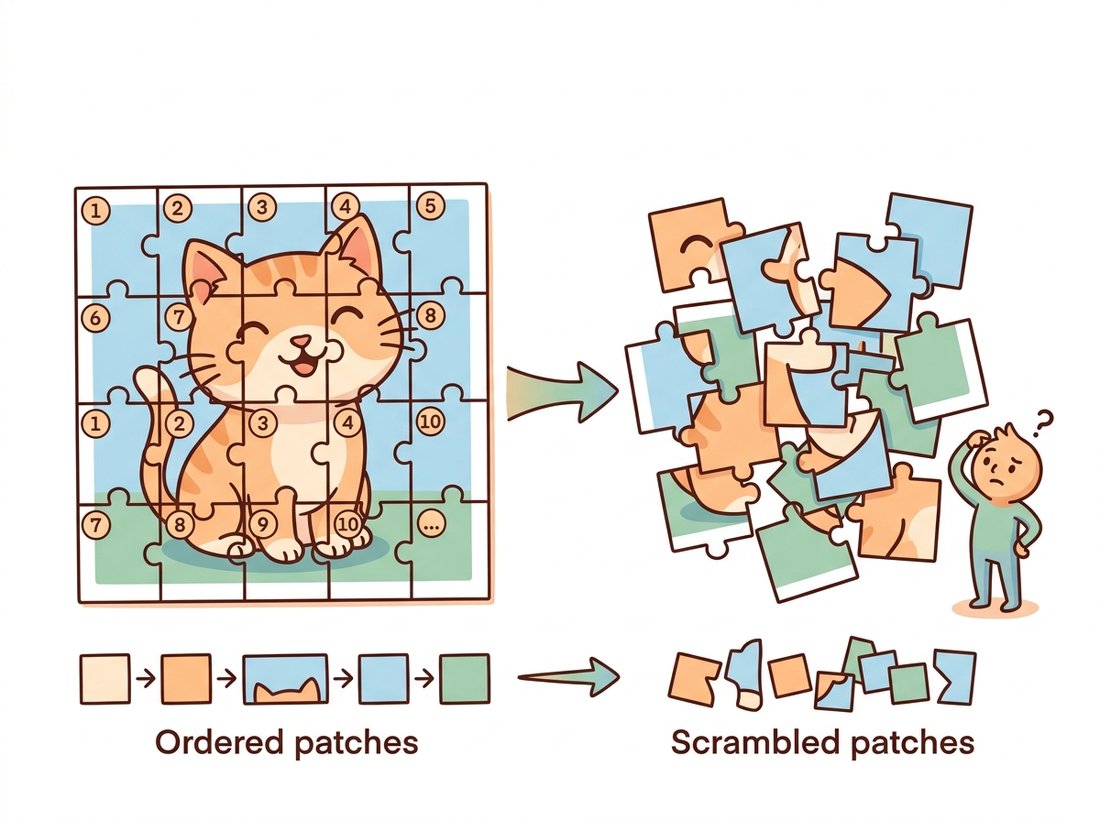
The second piece is positional embeddings, and they are not optional. Self-attention is permutation-invariant: shuffle the order of the tokens and the set of outputs is merely shuffled the same way, because attention treats its input as a set, not a sequence. That is fine for an unordered set, but an image is profoundly ordered; the patch in the top-left is not interchangeable with the one in the center. To restore spatial information, ViT adds a learned position vector to each token, one distinct vector per position. After this addition the token "knows" both what it contains and where it sits. The base ViT learns these position vectors directly as parameters; later designs use relative or 2D-aware schemes, but the principle is identical. Remove the positional embeddings and a ViT's accuracy collapses, because a cat reassembled from patches in random order is no longer a cat, as the illustration below makes vivid.

3. Assembling the Full ViT Intermediate

We now have every part: the patch embedding of subsection 1, the class token and positional embeddings of subsection 2, the transformer block of Section 22.1, and a final linear classification head. Assembling them gives the complete ViT. The forward pass reads exactly like the figure: embed patches, prepend the class token, add positions, run the encoder, take the class token's output, normalize, and classify. The code below reuses the TransformerBlock from Section 22.1.

# Full ViT-Base/16: patch embedding, a prepended learnable class token, learned
# positional embeddings, a stack of transformer blocks, then classify the final
# state of the class token alone. This reuses TransformerBlock from Section 22.1.
import torch
import torch.nn as nn

class VisionTransformer(nn.Module):
    def __init__(self, img_size=224, patch_size=16, in_chans=3, num_classes=1000,
                 embed_dim=768, depth=12, num_heads=12, mlp_ratio=4.0):
        super().__init__()
        self.patch_embed = PatchEmbed(img_size, patch_size, in_chans, embed_dim)
        n = self.patch_embed.num_patches
        # learnable class token and (n+1) positional embeddings
        self.cls_token = nn.Parameter(torch.zeros(1, 1, embed_dim))
        self.pos_embed = nn.Parameter(torch.zeros(1, n + 1, embed_dim))
        self.blocks = nn.ModuleList([
            TransformerBlock(embed_dim, num_heads, mlp_ratio) for _ in range(depth)
        ])
        self.norm = nn.LayerNorm(embed_dim)
        self.head = nn.Linear(embed_dim, num_classes)
        nn.init.trunc_normal_(self.pos_embed, std=0.02)
        nn.init.trunc_normal_(self.cls_token, std=0.02)

    def forward(self, x):
        B = x.shape[0]
        x = self.patch_embed(x)                          # (B, 196, 768)
        cls = self.cls_token.expand(B, -1, -1)           # (B, 1, 768)
        x = torch.cat((cls, x), dim=1)                   # prepend -> (B, 197, 768)
        x = x + self.pos_embed                           # add positions
        for blk in self.blocks:
            x = blk(x)                                   # L transformer blocks
        x = self.norm(x)
        return self.head(x[:, 0])                        # classify the class token

vit = VisionTransformer()
print("params (M):", round(sum(p.numel() for p in vit.parameters()) / 1e6, 1))
# params (M): 86.6   (this is ViT-Base/16)
print("logits:", vit(torch.randn(2, 3, 224, 224)).shape)  # torch.Size([2, 1000])

That is the entire architecture. The parameter count of about $86.6$ million is dominated by the twelve blocks, each carrying four projection matrices for attention and two large MLP matrices, exactly the per-block budget you can derive from Section 22.1. There is no pyramid, no pooling between stages, and no resolution change anywhere: every block sees the same $197$ tokens at the same width. That uniformity is part of the appeal (it makes scaling clean, as we will see in Section 22.5) and part of the inefficiency that Section 22.4 sets out to fix.

# Load a pretrained ViT-Base/16 plus the exact preprocessing its weights expect,
# so inference matches training without hand-coding the resize/crop/normalize.
import timm
model = timm.create_model("vit_base_patch16_224", pretrained=True).eval()
# the matching preprocessing (resize, crop, normalize) the weights expect:
cfg = timm.data.resolve_data_config({}, model=model)
transform = timm.data.create_transform(**cfg)
# logits = model(transform(pil_image).unsqueeze(0))

4. What the Encoder Actually Learns Advanced

It is natural to worry that a model with no locality bias would learn nothing sensible, yet trained ViTs develop structure that mirrors what CNNs learn, only reached differently. Analyses of trained ViTs (and the attention-rollout visualizations that aggregate attention across layers) show three consistent findings. First, lower blocks tend to attend locally, the model rediscovers that nearby patches are relevant, even though it could attend anywhere; higher blocks attend globally, relating distant regions. Second, the class token's attention in the final layers concentrates on the patches that actually contain the object, which is why those maps double as a rough, free segmentation. Third, the learned positional embeddings encode the 2D grid, as the fun fact above noted.

The practical lesson is that the inductive biases a CNN has built in, a ViT must learn, and it can learn them given enough data, but the words "enough data" are doing heavy lifting. That phrase is the entire subject of the next section. The decision of when to reach for a ViT therefore comes down to a question this section cannot answer alone: do you have, or can you borrow through pretraining, the data scale that lets the model learn the structure it was not given? Figure 22.2.1 and the code give you the architecture; Section 22.3 gives you the recipe that makes it trainable on the data most teams actually have.