"Global attention is wonderful until someone hands you a four-megapixel slide and asks for every cell nucleus. Suddenly talking to everyone at once is not enlightenment; it is a quadratic bill. So I learned to whisper in small rooms, then occasionally rearrange the furniture."
A Swin Transformer Who Discovered Windows
The plain ViT keeps one resolution and global attention at every layer, which is both quadratically expensive at high resolution and a poor fit for dense tasks that need multi-scale features; hierarchical transformers fix both by computing attention inside small local windows (linear cost) and by merging patches between stages to build a feature pyramid, recovering global reach by shifting the window grid between layers. The result is a transformer backbone that looks structurally like a ResNet, four stages of decreasing resolution and increasing channels, and that plugs directly into the detection and segmentation heads of Chapter 23 and Chapter 24. This section reintroduces, in learned form, the image-pyramid idea you first met classically in Chapter 4.
Section 22.1 warned that self-attention costs $O(N^2)$ in the number of tokens, and the document-pipeline example showed that wall in action. Section 22.2 noted the second problem: the plain ViT never changes resolution, so it has no natural way to produce the coarse-to-fine feature maps that object detectors and segmenters feed on. A ResNet hands a detector feature maps at 1/4, 1/8, 1/16, and 1/32 of the input resolution; a plain ViT hands it $196$ tokens at one scale and nothing else. Both problems have the same root, global single-scale attention, and Swin Transformer solves both with two ideas borrowed straight from the convolutional world: locality and a pyramid.
1. Window Attention: Locality, Reintroduced Beginner
The first idea is to stop attending globally. Swin partitions the feature map into non-overlapping windows (the default is $7 \times 7$ patches per window) and computes self-attention only within each window. A $7 \times 7$ window holds $49$ tokens, so a token attends to the $48$ others in its window plus itself, not to all several thousand in the image. This is a deliberate reintroduction of the locality bias that the plain ViT threw away, and it changes the cost from quadratic in the total token count to linear. If the image has $N$ tokens and each window holds $M$ tokens, global attention costs $O(N^2)$ while window attention costs $O(N \cdot M)$, and since $M$ is a small fixed constant the cost grows linearly with image size.
The saving is dramatic even at the very first Swin stage. A $56 \times 56$ token map holds $3136$ tokens, so global attention would build a score matrix of $3136^2 \approx 9.8$ million entries per head. The same map splits into $64$ windows of $49$ tokens, each with a $49^2 = 2401$-entry score matrix, about $154{,}000$ entries in total. That is a $64\times$ reduction at one stage, and because the number of windows grows with the image while their size stays fixed, the gap widens as the picture gets bigger. Writing multi-head self-attention as MSA, the two cost regimes contrast directly.
The catch is obvious: if every layer attends only within fixed windows, information never crosses a window boundary, and the model loses the global reach that made attention attractive in the first place. A token in the top-left window can never learn anything about the bottom-right. Swin's second idea solves exactly this.
2. Shifted Windows: Global Reach on a Budget Intermediate
The trick that gives Swin its name is the shifted window. In every other block, the window grid is displaced by half a window (in the default, by $3$ patches down and right) before attention is computed. Tokens that sat in separate windows in the previous block now share a window in this one, so information leaks across the old boundaries. Alternating a regular-window block with a shifted-window block, then stacking many such pairs, lets information propagate across the entire image after a few layers, while every individual attention computation stays local and cheap. It is the same logic as a CNN's growing receptive field, the field expands with depth, but achieved by relocating the windows rather than by enlarging a kernel. Figure 22.4.1 shows the shift.
The code below implements the core of window attention: partition into windows, attend within each, and reverse the partition. The shift itself is a torch.roll applied before partitioning and undone after, which Swin combines with a small attention mask so the rolled-around edges do not attend across the wrap. We show the window mechanics and describe the shift in comments to keep the example focused.
# Window attention plumbing: split a feature map into non-overlapping windows,
# attend inside each, then stitch them back. The commented roll/unroll pair is
# the shifted-window step that lets information cross window boundaries.
import torch

def window_partition(x, window_size):
    """x: (B, H, W, C) -> (num_windows*B, window_size, window_size, C)."""
    B, H, W, C = x.shape
    x = x.view(B, H // window_size, window_size, W // window_size, window_size, C)
    windows = x.permute(0, 1, 3, 2, 4, 5).reshape(-1, window_size, window_size, C)
    return windows

def window_reverse(windows, window_size, H, W):
    """Inverse of window_partition: (num_windows*B, ws, ws, C) -> (B, H, W, C)."""
    B = int(windows.shape[0] / (H * W / window_size / window_size))
    x = windows.view(B, H // window_size, W // window_size, window_size, window_size, -1)
    return x.permute(0, 1, 3, 2, 4, 5).reshape(B, H, W, -1)

# A shifted-window block first rolls the feature map, then partitions:
#   x = torch.roll(x, shifts=(-shift, -shift), dims=(1, 2))   # cyclic shift
#   windows = window_partition(x, window_size)                # attend per window
#   ... multi-head attention inside each window (with a roll-aware mask) ...
#   x = window_reverse(attn_windows, window_size, H, W)
#   x = torch.roll(x, shifts=(shift, shift), dims=(1, 2))     # undo the shift

x = torch.randn(2, 56, 56, 96)               # a Swin stage-1 feature map
w = window_partition(x, window_size=7)
print("windows:", w.shape) # windows: torch.Size([128, 7, 7, 96])The word "global" in the section title invites the belief that one shifted-window block lets any token see the whole image, the way a plain ViT block does. It does not. After a regular block followed by a shifted block, a token has exchanged information only with the windows it directly overlapped, so its effective reach has grown by roughly one window, not to the entire image. Global context in Swin is reached the same gradual way a CNN's receptive field grows: by stacking many block pairs so the reach compounds with depth. This is also why window attention is not simply a renamed convolution. Inside each window it is still full content-dependent attention (every token attends to every other token in the window with weights computed from the data), whereas a convolution applies the same fixed kernel regardless of content. Swin trades the plain ViT's immediate global reach for cheap locality, then earns the reach back over depth.
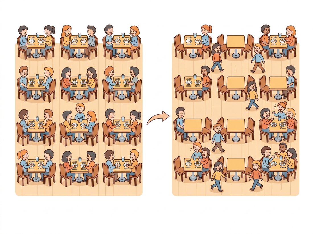
The shift is implemented not by re-cutting the grid but by sliding the whole feature map with a single torch.roll, attending in the same fixed windows, then rolling it back. The tokens move; the windows stay put. It is the computational equivalent of leaving the dinner tables bolted to the floor and asking half the guests to swap seats between courses, which is cheaper than rearranging the furniture. The signature phrase for the section: whisper in small rooms, then shuffle the seating. The illustration below makes the seat-swap concrete.
The plain ViT gave up locality (paying in data) and gave up multi-scale structure (paying in dense-task performance). Swin buys both back without abandoning attention. Window attention restores locality and makes the cost linear; the shifted windows recover global reach over depth, just as a CNN's receptive field grows over depth; and patch merging (subsection 3) restores the pyramid. The honest reading is that the most successful "vision transformer" reintroduced the very inductive biases the original ViT was celebrated for discarding. Attention is the engine, but the convolutional priors turned out to be worth keeping.
The linear-versus-quadratic claim becomes tangible with a one-line sweep, no training required. Take a fixed $56 \times 56$ token grid ($3136$ tokens) and, for each window size $M$ in $\{7, 14, 28, 56\}$, count the total score-matrix entries window attention builds: the number of windows is $(56/M)^2$ and each window's matrix has $M^2 \times M^2$ entries, so the total is $(56/M)^2 \cdot M^4 = 56^2 \cdot M^2$. Print that number for each $M$. Watch it climb from about $154{,}000$ entries at $M=7$ to roughly $9.8$ million at $M=56$, the full global-attention figure from subsection 1, a $64\times$ jump for an $8\times$ wider window. Then flip the experiment: fix $M=7$ and grow the grid from $56 \times 56$ to $112 \times 112$ and $224 \times 224$, and confirm the per-window cost stays flat while only the window count grows, which is exactly what makes the cost linear in image size rather than quadratic. The single dial that separates "fits on your GPU" from "out of memory" is the one you just turned.
3. Patch Merging: Building the Pyramid Intermediate
Window attention made the cost linear, but it left the plain ViT's other handicap untouched: one resolution, one scale, nothing for a detector to feed on. Why can a ResNet hand a detector four feature maps of different sizes while a plain ViT hands it exactly one? Because a ResNet changes resolution between stages and a plain ViT never does. The second structural fix is to change resolution between stages, the way a CNN does with strided pooling. Swin is organized into four stages. Between stages, a patch-merging layer concatenates each group of $2 \times 2$ neighboring tokens into one and applies a linear projection, halving the spatial resolution in each dimension and (typically) doubling the channel count. So the token grid goes $56 \times 56 \to 28 \times 28 \to 14 \times 14 \to 7 \times 7$ across the four stages, with channels $96 \to 192 \to 384 \to 768$, exactly the spatial-down, channels-up rhythm of Chapter 20. The four resulting feature maps are a genuine feature pyramid.
That pyramid is exactly what a dense-prediction head wants. The four maps are directly usable by a Feature Pyramid Network (FPN) detection head or a segmentation decoder. An FPN, which Chapter 23 covers in detail, is the standard module that fuses such multi-scale maps so a detector can find both large and small objects; here all that matters is that it expects exactly the several-scale maps Swin produces and a single-scale plain ViT does not.
This is the learned descendant of the Gaussian and Laplacian pyramids of Chapter 4. There, you built a pyramid by repeated blurring and downsampling to analyze an image at multiple scales; here, the network builds its own multi-scale hierarchy by merging tokens, and it learns what to keep at each scale rather than using a fixed Gaussian. Figure 22.4.2 contrasts the flat plain-ViT processing with Swin's four-stage pyramid.
Implementing the four stages, patch merging, relative position bias, and the shift masking correctly is several hundred lines. Both timm and torchvision ship Swin with pretrained weights and expose the pyramid feature maps for use as a detection or segmentation backbone:
# Use a pretrained Swin-Base as a multi-scale backbone instead of coding the
# four stages, shift masking, and patch merging by hand. The feature-extraction
# mode hands back the pyramid maps a detector or segmenter feeds on.
import timm
# features_only=True returns the four pyramid feature maps, ready for an FPN
backbone = timm.create_model("swin_base_patch4_window7_224",
                             pretrained=True, features_only=True)
feats = backbone(torch.randn(1, 3, 224, 224))
print([f.shape for f in feats]) # four maps at strides 4, 8, 16, 32features_only=True returns the four pyramid feature maps at strides 4, 8, 16, and 32, the multi-scale input a detection or segmentation head consumes directly.The library handles window partition and reverse, the cyclic shift and its attention mask, the relative position bias table, patch merging, and the stage configuration. The features_only=True flag is the production hook that makes Swin a drop-in backbone for the detectors of Chapter 23 and the segmenters of Chapter 24, where a single-scale plain ViT cannot directly fit.
4. The Pyramid Transformer Family Advanced
Swin is the most influential hierarchical transformer, but it is one member of a family that all reach the same destination, a multi-scale, near-linear-cost transformer backbone, by different routes. The Pyramid Vision Transformer (PVT, 2021) shrinks the token sequence stage by stage and uses spatial-reduction attention, which downsamples the keys and values before attention so the cost drops without windowing. Twins and other designs interleave local window attention with a cheap global attention to combine fine and coarse mixing. The Multiscale Vision Transformer (MViT) line, used heavily for video in Chapter 26, pools the queries, keys, and values to build the pyramid inside the attention itself.
The common thread is unmistakable. Every successful hierarchical transformer reintroduces some combination of locality, downsampling, and multi-scale structure, the priors a CNN has built in, while keeping attention as the mixing operator. This convergence is the central evidence for the argument of Section 22.5: the future is not "attention replaces convolution" but "attention and convolutional priors combine." The practical example shows a team navigating exactly this design choice.
Who: a mapping company segmenting buildings, roads, and vegetation from high-resolution aerial imagery, 2024. Situation: their tiles were $1024 \times 1024$ and the task was dense per-pixel segmentation, so they needed feature maps at several scales. Problem: a plain ViT-Base gave them a single $64 \times 64$ token grid (with $16 \times 16$ patches) and no pyramid, so their FPN-style decoder had nothing multi-scale to consume, and raising the resolution hit the $O(N^2)$ wall from Section 22.1. Decision: they swapped to a Swin-Base backbone with features_only=True, which produced feature maps at strides 4, 8, 16, and 32, feeding the decoder directly, and whose window attention kept the $1024 \times 1024$ tiles within memory. Result: segmentation of thin structures like roads improved markedly because the stride-4 map preserved fine detail, and the model trained on the same GPUs that had refused the high-resolution plain ViT. Lesson: for dense prediction at high resolution the backbone choice is dictated less by raw classification accuracy than by whether it produces a usable pyramid at affordable cost, which is precisely what the hierarchical designs of this section were built to deliver.
By 2023 to 2025 two counter-currents complicated the hierarchical story. First, ConvNeXt (Liu et al., 2022, arXiv:2201.03545) and ConvNeXt V2 (2023) showed a pure CNN, modernized with transformer-era training and design choices, matches Swin on the same detection and segmentation benchmarks, suggesting the hierarchy mattered more than the attention. Second, the "plain ViT as a backbone" line, especially ViTDet (Li et al., 2022, arXiv:2203.16527), demonstrated that a single-scale plain ViT can be turned into a strong detector by building a simple pyramid only at the very end, with a few deconvolution and pooling layers, rather than baking the hierarchy into every stage. The unresolved 2025 question is how much of Swin's advantage came from windowed attention versus from simply having a pyramid at all, and ViTDet's success argues that the pyramid, however it is produced, is the load-bearing ingredient.
Imagine a Swin variant that uses window attention but never shifts the windows. Describe what happens to information flow across window boundaries as you stack more blocks, and argue why this network's effective receptive field would stay stuck at the window size no matter how deep it is. Then explain, using Figure 22.4.1, how a single half-window shift between two blocks lets a token in one window influence a token in a diagonally adjacent window after just two layers. Relate the argument to the growing-receptive-field discussion of Chapter 19.
Write a small script that, for token-grid sizes from $14 \times 14$ up to $112 \times 112$, computes (a) the number of score-matrix entries for global attention ($N^2$) and (b) the number for $7 \times 7$ window attention (number of windows times $49^2$). Plot both against grid size on a log-y axis. Confirm that global attention curves up quadratically while window attention is a straight line (linear). Then estimate at which grid size the global attention matrix would exceed, say, 8 GB of memory in float32 for a single head, and connect the answer to the document-pipeline and aerial examples.
Load a pretrained Swin backbone with features_only=True as in the library shortcut and run it on a $224 \times 224$ image. Print the shape of each of the four feature maps and verify the strides (4, 8, 16, 32) and the channel doubling. For one map at an intermediate stage, visualize a few channels as heatmaps and describe qualitatively what scale of structure each stage seems to capture (fine edges versus object-level regions). Compare this to the multi-scale Gaussian pyramid of Chapter 4 and note one difference between a fixed Gaussian pyramid and this learned one.